Lecture 11

2025-07-21

Case Study: European Football Player Valuation: Integrating Financial Models and Network Theory

Albert Cohen and Jimmy Risk

Acknowledgement

This lecture is taken from a presentation by Dr. Cohen on March 7, 2025 at the Simon Fraser University Sports Analytics Group Virtual Seminar Series. That recording can be found HERE and the companion code to the paper HERE

Pay and Performance in Soccer

• Player valuation in European football is a complex endeavor, requiring nuanced metrics that go beyond traditional sports statistics

• Due to the dearth of goals in a game, other in-game events should be utilized to understand the contrbution of individual players to the team’s performance

• Existing methods often fail to capture the dynamic, stochastic nature of player performance and its impact on fair market valuation.

Pay and Performance in Soccer

The authors introduce a multi-disciplinary approach that integrates financial models with stochastic player performance models, borrowing from social network theory. Their main objectives are

1. Formulate a player valuation model that integrates the passing matrix with financial mathematics, specifically stochastic asset pricing models, and
2. Validate this integrated model empirically through a case study involving real-world data

Stochastic asset pricing models are mathematical frameworks used to describe how the prices of financial assets evolve over time under uncertainty. These models incorporate randomness (stochastic processes) to reflect the unpredictable nature of markets.

Linking Pay with Performance

The authors identify at three foundational works that have provided in-depth analyses of various pieces of this puzzle:

• The first major work to address the link between performance and pay for athletes can be found in the paper of Scully (1974)

• In this paper, the author investigated the connection between a baseball team’s revenue and the salary paid to the team’s players. By utilizing well-known tools in labor economics, such as the marginal revenue product (MRP) related to units of labour, the author derived a framework to link on-field play with salary.

Aside: Marginal Revenue Product (MRP)

• Classical economic theory suggests that a profit maximizing firm will hire by setting wage equal to marginal revenue product of labor, which is the increase in revenue attributable to a unit increase in labor

• A common sports analytics application is that a player should be compensated in relation to their contribution to team performance.

  • Specifically, the player should be paid relative to each extra dollar of revenue they generate due to their performance on the team, related to their marginal effect on winning percentage

this is not fully sufficient for player valuation. For example, Rockerbie and Easton (2020) [Chapter 2] finds that in baseball, higher-priced free agents are overpaid relative to their MRP, while lowerpaid free agents offer a bargain. The cause for this could be for a variety of reasons, one being that paying MRP as wage holds true when teams are profit-maximizing (Rosen and Sanderson 2001), but not necessarily when teams are win-maximizing. Késenne (2000) find that in European football clubs, win-maximizers can result in different revenues and payroll than under profit maximization.

Linking Pay with Performance

• The second major work referenced by the authors is that of Tunaru, Clark, and Viney (TCV) (2005), which addressed the value \(V\) of a player to a team, in continuous-time, via stochastic modeling and a subsequent Black-Scholes partial differential equation (PDE).

• The solution \(V\) of that PDE also includes the assumption that contracts can be sold at the end of the term

  • There have been some numerical implementations of this model, such as estimating the value of a goalkeeper to a Serie A league club (Coluccia, Fontana, and Solimene 2018)

Aside: Black-Scholes Partial Differential Equation

A Black-Scholes partial differential equation is used to model changes in the value of options (rights to buy and sell assets) over time, written as

\[ rS_t\frac{\partial V}{\partial S} + \frac{\partial V}{\partial t} + \frac{1}{2}\sigma^2 S^2 \frac{\partial^2 V}{\partial S^2} -rV = 0 \]

Here, \(V\) is the value of the option at time \(t\) with underlying asset price \(S\), \(r\) is the risk-free interest rate, and \(\sigma\) is the volatility of the underlying asset.

The equation balances the change in the option price over time with the risk and return of holding the option. 

Aside: TCV Modeling approach

Let \(T\) be the turnover for the club, \(N\) be the number of Opta Index points for the individual player under evaluation, \(S\) be the sum of Opta Index points for all players playing for the club.

• Then it follows that \(X=T/S\) is the value in money for the club of a single Opta Index point and \(Y=N⁢X\) is the Opta value of the player.

Aside: TCV Modeling the value of the player as a jump-diffusion process

Financial modelling can be adapted to deal with the assumption that the jumps affect directly the evolution of the underlying.

• Here, one can argue that \(N\), that is the number of Opta Index points for the player under evaluation, is a time series that experiences downward jumps when that player has injuries.

The authors assume that the turnover \(T\) and the Opta value of the team \(S\) follow correlated geometric Brownian motions, see Neftci (1996). d⁢T=α⁢T⁢d⁢t+σ⁢T⁢d⁢z d⁢S=γ⁢S⁢d⁢t+δ⁢S⁢d⁢w E(d⁢S⁢d⁢T)=ρ⁢d⁢t

Linking Pay with Performance

• Finally, the work of Rockerbie and Easton (2020) in their recent book offers a discrete, multi-period approach to contract pricing via expected present valuation and cohort analysis via a market beta.

  • They also consider the real-option value of a player re-signing between seasons, which isn’t addressed in the current work

Linking Pay with Performance

• In applying the principle of linking pay to a player’s MRP, the authors of this paper seek to connect the discrete landscape of Rockerbie and Easton with the continuous stochastic modeling of Tunaru, Clark, and Viney by defining a player peformance share as a stochastic process correlated to a team’s revenue.

• The continuous-time TCV model proposes that a player’s performance is measured by a point (or performance) score that lives on the interval (0, \(\infty\))

Linking Pay with Performance

• The authors model this score for player \(j\) as a geometric Brownian motion (GBM) \(p_j\) that is correlated to another GBM in \(R\) that models the team’s revenue.

  • The authors make a simplifying assumption that the sum over player \(\sum_j p_j\) itself follows a GBM

• The result is that the revenue earned, per point, by the team is \(R/\sum_j p_j\) and the number of points \(n\) that multiplies this fraction returns the performance-linked value of player \(j\) to that club, \(Z_j := p_j R/\sum_j p_j\)

\(R\) is revenue

\(p_j\) is the non-standardized index point value of player j.

The reason for writing it this way is because \(R_t∕ \sum_i q_i\),t is value in money for a single point of the team.

Aside: (Geometric) Brownian Motion

• A standard Brownian Motion \(W(t)\) is defined on \(0 \leq t \leq T\) as

• A stochastic process \(S(t)\) follows a geometric Brownian motion if it satisfies this stochastic differential equation (SDE)

\[ dS(t) = \mu S(t) + \sigma S(t)dW(t) \]

• We apply this to treat a player’s transfer market value like a financial asset price

• S(t): the asset price at time t

• μ: the drift term (expected return)

• σ: the volatility (standard deviation of returns)

• W(t): a standard Brownian motion

• dW(t): the random component, representing unpredictable market movements

This is the foundation of the aforementioned Black-Scholes model

🔍 Intuition

• The drift μ pulls the price upward over time (like an average growth rate).

• The volatility σ introduces randomness, causing the price to fluctuate.

• The multiplicative nature (i.e., S(t) multiplied by both μ and σ) ensures that prices remain positive and exhibit log-normal behavior.

Linking Pay with Performance

The authors propose linking this stochastic model to that of Rockerbie and Easton by rewriting the performance linked value \(Z_j\):

\[\begin{equation} \label{eq:perf} \tag{1} Z_j = p_j \cdot \frac{R}{\sum_j p_j} = \frac{p_j}{\sum_j p_j} \cdot R : = \pi_jR \end{equation}\]

• Here, the dynamic \(\pi_j = \frac{p_j}{\sum_j p_j}\) models the normalized performance share that a player provides with their on-field play.

Linking Pay with Performance

• For example, in soccer if one simplifies to think of 11 key players, a uniform distribution of performance load would suggest that each player would provide \(\pi_t = 1/11 = 0.0909\) per game

• This obviously does not happen, as there are injuries, substitutions, matchups that enhance or detract from a specific player’s ability to contribute, and even worries about upcoming contract negotiations, to name a few (of a multitude of factors).

Linking Pay with Performance

• Finally, there are many in-game decisions that can lead to performance estimation, and this requires the special attention of analytics providers that may keep such metrics away from public view.

• To address these and other issues, the author’s model can be calibrated using publicly available data

• In doing so, they compute (augmented) passing matrices derived from in-game stats to apply network analysis methodologies similar to that of Pena and Touchette (2012) and Duch et.al. (2010; 2015)

New SDE Model for Player Salary Valuation

• Applying network theory allows us to define, according to managerial input, what drives performance share. Once this is established, we can calibrate the model in (Rockerbie and Easton 2020) below:

• Consider the univariate approach of a single player \(j\).

• Thus, we need to determine the evolution of \(Y_t = \pi_ta_tR_t\), which appears as the product of the two stochastic variables \(\pi\) and \(R\), with an update for a dynamic fraction \(a_t\) that represents the portion of revenue set aside for player salaries.

• \(a_t\) is the proportion of team revenue that goes to players at time t.
• \(π_j\),t ∈ (0, 1) is player j’s team-standardized performance index at time t, and
• \(R_t\) is the revenue at time \(t\).

In what follows we assume at is known ahead of time, effectively encoding information about whether the club is a win-maximizer (larger \(a_t\)) or profit-maximizer (smaller \(a_t\)).

Connection with Passing Matrix

• To value scoring attempts and devalue missed passes and turnovers, the authors augement the passing matrix wth two rows and columns: one for shots (\(S\)) and another for unsuccessful passes and/or turnovers (\(U\)).

• This augmented passing matrix is denoted by \(P\). Here, “shots” can refer to successful shots, total shots, or a weighted combination of successful shots and missed shots.

Connection with Passing Matrix

• Thus, \(P\) is a \((M_2) \times (M+2)\) transition probability matrix of a Markov chain with two absorbing states (\(S\) and \(U\)), where, for \(1 \leq i, j\leq M\), \(p_{i,j}\) is the probability that, if player \(i\) has the ball, they pass to player \(j\).
  • \(p_{i, S}\) is the probability of transitioning to the \(S\) state, and
  • \(p_{i,U}\) is the probability of an unsuccessful pass.

Example

\[ P = \left[ \begin{array}{ccccccc} 0 & 0.40 & 0.25 & 0.20 & 0.10 & 0 & 0.05 \\ 0.15 & 0 & 0.34 & 0.25 & 0.10 & 0.01 & 0.15 \\ 0.05 & 0.15 & 0 & 0.20 & 0.30 & 0.05 & 0.25 \\ 0.05 & 0.15 & 0.20 & 0 & 0.20 & 0.10 & 0.20 \\ 0 & 0 & 0.25 & 0.25 & 0 & 0.15 & 0.30 \\ 0 & 0 & 0 & 0 & 0 & 1 & 0 \\ 0 & 0 & 0 & 0 & 0 & 0 & 1 \\ \end{array} \right] \]

For example, the first row corresponds to the goalkeeper (A), who has respective probabilities 0.4, 0.25, 0.2, and 0.1 of passing to players B, C, D, E. The goalkeeper has probability 0 to directly transfer ball possession to the S state (6th column), and has probability 0.05 of making an unsuccessful pass or turnover. Note that each row sum is 1. The rows are presented in order of field position, so player B is a defender, players C and D are wing playmakers, and player E is the primary scorer. Note that the probability of leaving state S is 0, and the same is true for state U (missed passes and/or turnovers), since the team possession ends when the ball reaches that state.

Connection with Passing Matrix

• Further, \(p_{S,S} = p_{U,U} = 1\) as \(S\) and \(U\) are considered terminal states. Here, each team ball possession is considered a realization of the Markov chain where the state is which player has the ball at that time.
• The quantity of interest is

\[\begin{equation*} q_j = \mathbb{P}[\text{player } j \text{ is involved in possession} \mid \\\text{possession ends in }S \text{ not } U] \end{equation*}\]

Connection with Passing Matrix

• Extreme cases provide some quick insight: if \(q_j = 1\), it means all shots were filtered through player \(j\) in some manner. Similarly, \(q_j=0\) means that player \(j\) is not involved in any possession that ended in a shot.

• Even for strong defensive players, we would still expect \(q_j\) to be relatively large, as many shot-based possessions will involve them beginning with the ball.

Connection with Passing Matrix

In order to relate to the \(\pi_t\) process,

1. Assume the passing matrix varies over time. Thus we write \(q_{i,t}\) for player \(i\)’s probability of involvement at time \(t\). Here, \(t\) could be per game or season
2. Define for each \(t\) and player \(j\)

\[ \pi_{j,t} = \frac{q_{j_t}}{\sum_iq_{i,t}} \]

Connection with Passing Matrix

• Note here we emphasize the subscript \(\pi_{j,t}\), instead of \(\pi_t\) as we are comparing across players on the team.

• This ensures \(0\leq \pi_{j,t} \leq 1\) and transforms \(q_{j,t}\) into a measure of relative player importance.

New SDE Model for Player Salary Valuation

• The authors present their model extension here for the value \(Y\) attributed to performance:

\[\begin{equation} \begin{aligned} Y_t &= \pi_t a_t R_t \\ d\pi_t &= -\theta(\pi_t - \pi^*)dt + \sigma_\pi \sqrt{\pi_t (1 - \pi_t)}\, dW_t^{\pi} \\ dR_t &= \mu_R R_t\, dt + \sigma_R R_t\, dW_t^{R} \\ \rho\, dt &= \langle dW_t^{\pi}, dW_t^{R} \rangle \end{aligned} \tag{4} \end{equation}\]

These are the dynamics of the continuous time models.

where σR, σπ, θ > 0, −1 ≤ ρ ≤ 1, 0 ≤ π∗ ≤ 1, and min(π∗, 1 − π∗) ≥ σ2π∕(2θ). Here, Wπ and WR are Brownian motions (Shreve et al. 2004) with correlation ρ as indicated in the last line of (6). Note that R follows a geometric Brownian motion (GBM) (Shreve et al. 2004) with growth rate μ and volatility σR. The process defined by πt lies in the family of Pearson diffusion processes (Forman and Sørensen 2008). These have well known properties. To name a few, πt is guaranteed to be bounded on (0,1) and πt has stationary (long-term) distribution Beta with known parameters in terms of θ, π∗, and σπ (Bakosi and Ristorcelli 2010). The parameter θ controls the rate of reversion to the stationary mean π∗, which can be seen through

New SDE Model for Player Salary Valuation

• Here, \(a_t\) is the proportion of team revenue that goes to players in year \(t\).
• The process defined by \(\pi_t\) lies in the family of Pearson diffusion processes. These have well known properties.
  • To name a few, \(\pi_t\) is guaranteed to be bounded on \((0,1)\) and
  • \(\pi_t\) has stationary (long-term) distribution Beta with known parameters in terms of \(\theta, \pi^*, \text{ and } \sigma_\pi\)

Discretization Over Smaller Periods

• Consider a scenario where a player can sign a contract with a team for multiple years, with

  • the negotiated salary payments, \(C_1, C_2, \ldots, C_T\) with the amount \(C_t\) computed as if paid at the end of the \(t^{\text{th}}\) year, and

  • the random dollar-value of the athlete’s performance-linked contributions on the field, \(Y_1, Y_2, \ldots, Y_T\).

• There is a baseline expectation for performance, but management allows for the possibility that the player can under- or over-perform, in terms of expected statistical contribution

Discretization Over Smaller Periods

• We seek to find a balance, or swap, of fixed salaries for unknown performance values. The performance-shared payment schemes and performance-shared payment schemes should be equal, that is,

\[ \sum_{t=1}^Te^{-rt}C_t=\sum_{t=1}^Te^{-(r+\lambda)t}\mathbb{E}_0[Y_t] \]

Midterm Check-in

• To see how a contract negotiated at time 0 has aged by the middle of the term, we define the time \(t\) valuation of a player \(j\)’s performance-linked value as \(S_{t,t+h}\).

• In words, this is the new (rolling) value of a fixed contract if the manager could re-negotiate with a single payment at time \(t\) and single stochastic valuation at time \(t+h\).

• For such a 1-period swap, the agreed upon time \(t\) value at time \(t+h\) is \(S_{t,t+h}\), where

\[ e^{-rh}S_{t,t+h}=e^{-(r+\lambda)h}\mathbb{E}[Y_{t+h}\mid\mathcal{F}_t] \]

Flexible Contract Valuation

Consider a case where a player’s agent has asked for a three-year contract where

• the salary is front-loaded with year 1 salary \(C_1\) triple that of years 2 and 3, i.e. \(C_1 = 3C_2 = 3C_3\), which could act as a signing bonus,

• the risk-free rate \(r\) is set at the current 3-year UK government bond rate of \(r = 0.0375\),

• an agreed-upon risk-premium of \(\lambda = 0.01\), and

• a constant fraction of \(a_1 = a_2 = a_3 = 0.5\) of revenue directed towards player salaries over the next three years.

Flexible Contract Valuation

Additionally,

• initial revenue \(R_0 = 100\) (in \(\text{ €}1,000,000\)) and performance share \(\pi_0 = 0.08\)

• long-run performance expectation \(\pi^* = 0.10\)

• correlation between revenue and performance fraction set at either (a) \(\rho = 0\) or (b) \(\rho = 0.30\),

• corresponding (R,\(\pi\)) volatilities fixed at \((\sigma_{\text{R}}, \sigma_\pi)\) = (0.20, 0.25), mean reversion rate of \(\theta = 4\)), and a growth rate \(\mu = 0.10\) for the team’s revenue

Flexible Contract Valuation

Applying our swap model, the resulting balance equation for the full contract is now

\[\begin{equation} e^{-r}(3C) + e^{-2r}(C) + e^{-3r}(C) = e^{-r} S_{0,1} + e^{-2r} S_{0,2} + e^{-3r} S_{0,3} \tag{8} \end{equation}\]

Plugging in \(r = 0.0375\), the year 2 and 3 salaries \(C\) can be solved to be:

\[\begin{equation} C = \frac{e^{-0.0375} S_{0,1} + e^{-0.0375(2)} S_{0,2} + e^{-0.0375(3)} S_{0,3}}{3e^{-0.0375} + e^{-0.0375(2)} + e^{-0.0375(3)}} \tag{9} \end{equation}\]

Flexible Contract Valuation

Now, using the parameters described on the previous slide, we can use Taylor Series to approximate \(\{S_{0,1},S_{0,2},S_{0,3}\}\)

1. For the case of \(\rho = 0\), equation (9) returns \(C = 3.5349\) (in millions of pounds), resulting in a contract term structure proposal to the player of

\[ (C_1, C_2, C_3) = (10.6046, 3.5349, 3.5349) \]

Flexible Contract Valuation

2. For the case of \(\rho = 0.30\), a similar calculation yields \(C = 3.5745\) and it follows that

\[ (C_1, C_2, C_3) = (10.7236, 3.5745, 3.5745) \]

The authors emphasize here that numerical methods for pde’s could also be used to solve for the values \(\left\{e^{-\lambda j}\mathbb{E}[Y_j\mid\mathcal{F}_0]\right\}^3_{j=1}\) detailed in the swap (8).

Flexible Contract Valuation

The authors make the following observations:

• The salaries \((C_1,C_2,C_3) \mid_{\rho=0.30} > (C_1, C_2,C_3) \mid_{\rho=0}\).

• This would coincide with rewarding a player whose increased contributions have a positive effect on team revenue. A general formula for the corresponding “Greek” \(\frac{\partial \text{C}}{\partial \rho}\) would be interesting and valuable in player-team negotiations, and is the subject of further research.

• A player agent would be expected to argue that their client’s performance over the proposed contract has at least some partial (positive) correlation (i.e. \(\rho > 0\)) with team revenue

Case Study: 2018-2023

• Assume \(\rho = 0.30\) for the \(K= 5\) seasons considered

• Revenue data, available annually, is from Deloitte

• Salary data from Sportrac

• Game data is from Whoscored

• Game appearance data is from Transfermarkt, and is available for every game over the seasons of interest

Case Study: Notes

Liverpool:

• Mohamed Salah (right winger), the team’s primary offensive threat;

• Trent Alexander-Arnold (right-back), recognized for his creative playmaking; and

• Virgil Van Dijk (center-back), known for his defensive stability and leadership.

All players were starters for the considered seasons.

Case Study: Notes

Arsenal

• Eddie Nketiah (striker), a young goal poacher;

• Granit Xhaka (central midfielder), a key figure in controlling the game’s tempo; and

• Rob Holding (center-back).

Granit Xhaka was the only consistent starter for all seasons.

Case Study: Notes

Brighton

• Pascal Gross (attacking midfielder), the team’s creative engine;

• Solly March (winger/full-back), valued for his versatility and work rate; and

• Lewis Dunk (center-back), the cornerstone of Brighton’s defense.

All players were starters for the considered seasons.

Case Study: Notes

• With a variety of teams and consistency of positions, these players provide a practical basis for validating the estimates.

• The contributions in different positions provide a comprehensive view of the dynamics of \(\pi_t\) over time, reflecting both the offensive and defensive aspects of the game.

• Additionally, it considers players who are not starters as well as a team lacking superstars (Brighton).

Case Study: Estimated Player Parameters

Data are collected per game and player shares are statistically estimated

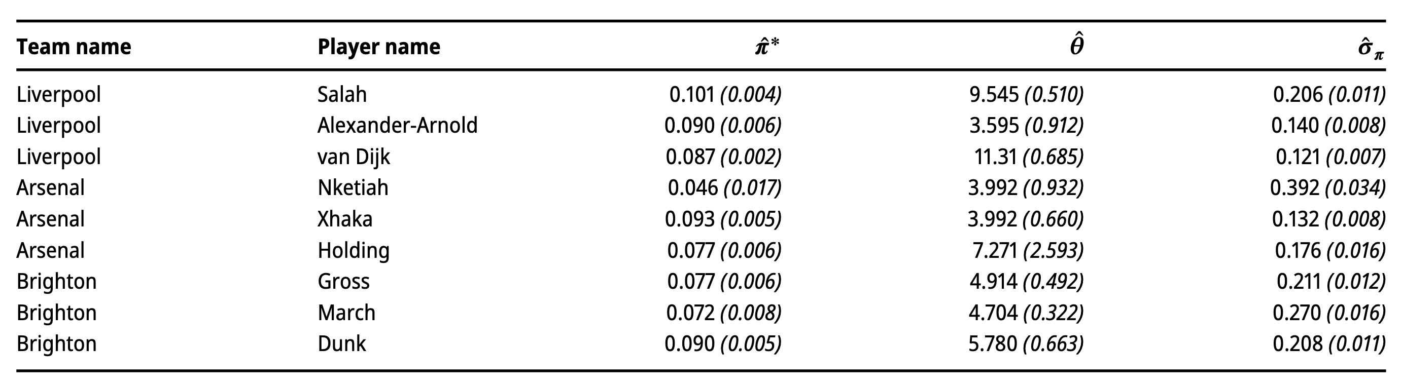
Estimates related to the performance share process for each player under analysis. The quantity in parentheses is the standard error of the estimate. Game-specific data is from https://www.whoscored.com

Salah is above the 0.091 average \(\pi*\) - long term expected averages. not every player contributes over 9.1% out of the starting 11, then the mean reversion parameter(Speed of mean reversion (rate at which the process is pulled back toward \(\mu\)))

Case Study: Estimated Player Parameters

Table: Estimates of risk premium \(\hat{\lambda}\) over players. Trent refers to Trent Alexander-Arnold.

this is particularly interesting for the act sci and quant people, Salah is 1% lambda, but everyone else is quite high, meaning that they have particularly high risk premiums that they would demand, so we gotta keep that in mind for discounting and therefore a better actuarial estimate of game readiness woudl be valuable.

Case Study: Estimated Team Parameters

• If the full revenue data were available, all parameters could be estimated more accurately, including a more precise estimation of \(\rho\).

• Similarly, the player share \(a_k\) over season \(k\) should practically be known from the club’s financial statements.

• As these data are unavailable, we estimate it as the historic fraction that went out to the club’s players over season \(k\) for each season.

Case Study: Estimated Team Parameters

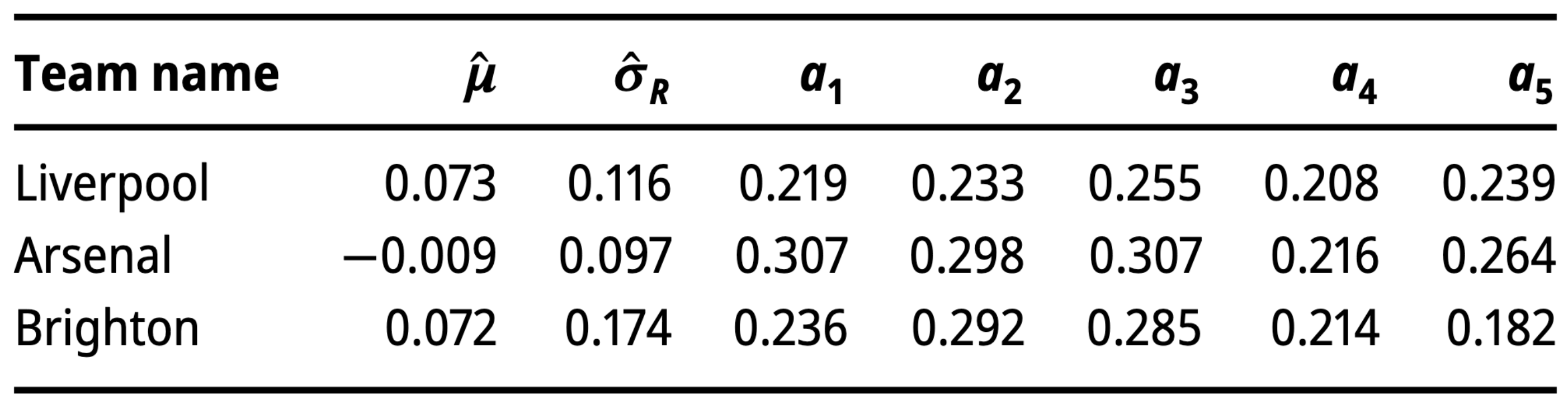
Estimates of \(\pi\), \(\sigma_R\) and calibrated values for each team’s player share \((a_k)\) process.

mu is the yearly growth, with low sigmas. Looking at the sharpe ratios for each of the teams could be interesting

the revenue shares year over year are ~20-30 percent, which is less than the 50% that you see in capped leagues

Case Study: Notes

For the figures on the next two slides:

• 1st slide: Calculated \(\pi_t\) processes using historical game data. The thick dark line is the average over that season, and the dashed line is reference of \(1/11 \approx 0.0909\), the share if a team consisted only of starters each with equal share

• 2nd slide: Time \(t\) on x-axis, \(\text{\$}1,000,000\) (annually) on y-axis. Plotted are \(C_t\) (thick dark line) and \(S_{t,T}\) (colored time series plots), where \(T = 1,2,\ldots,5\) represents seasons, and \(T-1 \leq t < T\) for each season.

Numerical Results: Performance Share:

See Figure 1 of (Cohen and Risk 2025)

Talk about salah, well above 0.9 and ver consistent

talk about Nketiah variability

Granit-Xhaka: performance shares decrease over time, but is pretty consistent

From a coaching perspective this is useful for how they play in terms of driving successful passing

Numerical Results: Valuation

See Figure 2 of (Cohen and Risk 2025)

true salary vs fixed salary

salah overperformed the fixed contract. Then he gets a massive contract and is underperforming relative to that contract

Eddie - underperforms in terms of performance, but overperforms in terms of dollars being paid.

Other that Salah and Van Dyk, most players are undervalued according to this model. This is due to liquidity, we overpay to keep a player that we don’t want to leave. so he’s the opposite of eddie

Discussion

• The valuation model reveals significant patterns in how player compensation aligns with performance, highlighting both consistencies and discrepancies within current salary structures in European football.

• Several players were consistently undervalued relative to their contributions before receiving pay increases.

Discussion

• For example, Mohamed Salah’s performance data from 2018-2021 suggested a need for a substantial pay increase.

  • He received a significant salary increase in the 2022-2023 season, which addressed his previous undervaluation. However, this increase appears to exceed what his performance metrics justify for that period

• Indeed, his value was higher in 2022-2023 but still below the salary provided, indicating a possible overvaluation, or most likely factors not considered in the model.

Discussion

• Trent Alexander-Arnold was under-compensated until the 2020-2021 season; his significant pay raise in 2021-2022 aligns with our model’s valuation. However, he continues to outperform his compensation, suggesting that he remains undervalued even after the increase

• Granit Xhaka also consistently demonstrated performance exceeding his compensation. The minor salary increase he received in 2022-2023 does not fully reflect his contributions, indicating that he is still undervalued according to the model.

Discussion

• Players such as Virgil van Dijk exhibit a close alignment between compensation and performance. He received a minor salary increase, and his compensation generally matches his performance value throughout the evaluated seasons.

Future Work

• Proposed approach that expands mapping \(\text{performance} \rightarrow \text{salary}\) to \(\text{performance} \rightarrow \text{revenue} \rightarrow \text{salary}\)

• Is there a dynamic Pythagorean exponent that could perhaps help with some of this analysis?

• Could closeness centrality measures be used to imply the ratio of offense to defense in a team?

References

Clemente, Filipe Manuel, Micael Santos Couceiro, Fernando Manuel Lourenço Martins, and Rui Sousa Mendes. 2015. “Using Network Metrics in Soccer: A Macro-Analysis.” Journal of Human Kinetics 45 (April): 123–34. https://doi.org/10.1515/hukin-2015-0013.

Cohen, Albert, and Jimmy Risk. 2025. “European Football Player Valuation: Integrating Financial Models and Network Theory.” Journal of Quantitative Analysis in Sports 21 (1): 3–22. https://doi.org/10.1515/jqas-2024-0006.

Coluccia, Daniela, Stefano Fontana, and Silvia Solimene. 2018. “An Application of the Option-Pricing Model to the Valuation of a Football Player in the ’Serie a League’.” International Journal of Sport Management and Marketing 18 (1-2): 155–68. https://doi.org/10.1504/IJSMM.2018.091345.

Duch, Jordi, Joshua S. Waitzman, and Luís A. Nunes Amaral. 2010. “Quantifying the Performance of Individual Players in a Team Activity.” PLOS ONE 5 (6): e10937. https://doi.org/10.1371/journal.pone.0010937.

Peña, Javier López, and Hugo Touchette. 2012. “A Network Theory Analysis of Football Strategies.” https://doi.org/10.48550/arXiv.1206.6904.

Rockerbie, Duane W, and Stephen T. Easton. 2020. Contract Options for Buyers and Sellers of Talent in Professional Sports. Palgrave Pivots in Sports Economics. Cham: Springer International Publishing. https://doi.org/10.1007/978-3-030-49513-8.

Scully, Gerald W. 1974. “Pay and Performance in Major League Baseball.” The American Economic Review 64 (6): 915–30. https://www.jstor.org/stable/1815242.

Tunaru, Radu, Ephraim Clark, and Howard Viney. 2005. “An Option Pricing Framework for Valuation of Football Players.” Review of Financial Economics, Real options SI, 14 (3): 281–95. https://doi.org/10.1016/j.rfe.2004.11.002.

Next Up

• Module 4: Web Applications and Dashboards
  • Mastering Shiny: 13-16
• Last class of the semester: Friday, July 25 at 2pm in M3 4206
  • Guest lecture by Dr. Jack Davis