Lecture 12

2025-07-25

Case Study: MBI and Beyond

Dr. Jack Davis, University of Waterloo

Outline

• Preliminaries
• What is MBI?
• What’s the problem
• What can we do instead?

Preliminaries: The Problems with P-Value

• First what is the p-value, and why do people hate it? P-value refers to the probability of obtaining at least as extreme evidence against your current null hypothesis if that null hypothesis is actually true.

• There are some complications with the definition. First, “as extreme” needs to be further clarified with a one-sided or two-sided alternative hypothesis. Another issue comes from the fact that you’re dealing with a hypothesis as if it’s already true.

Preliminaries: The Problems with P-Value

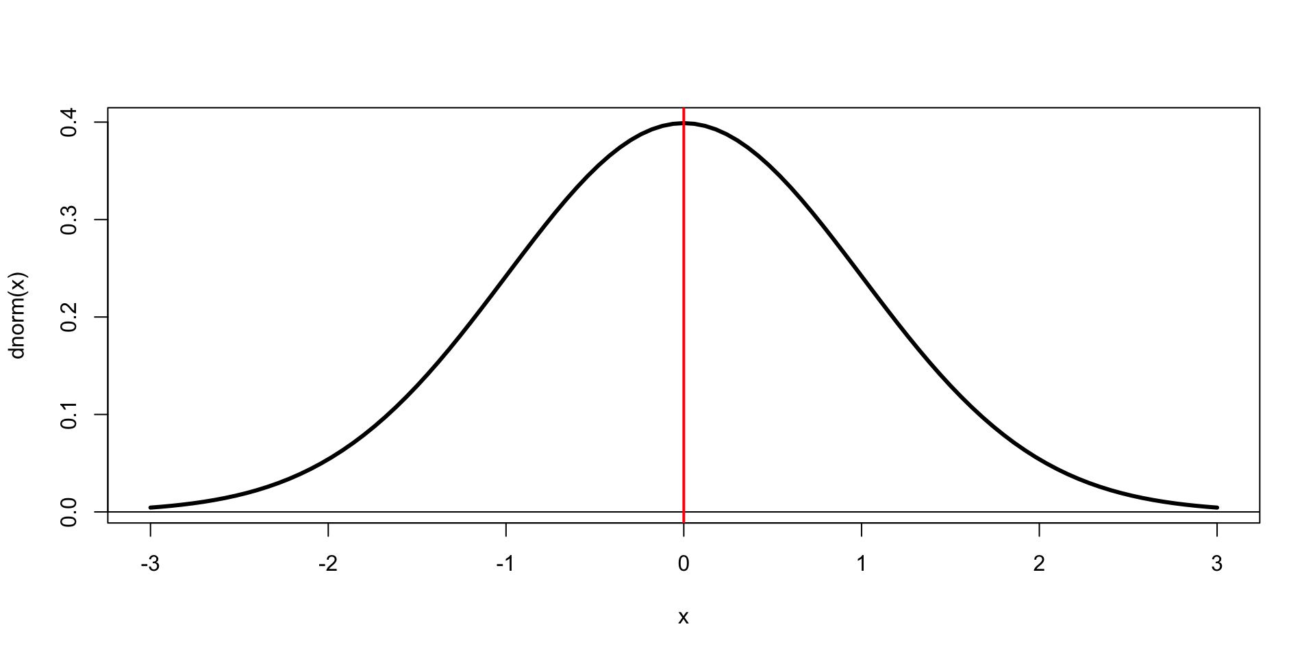
• If the parameter comes from a continuous distribution, the chance of it being any given value is zero, so we’re assuming something that is impossible by definition. If we are hypothesizing about a continuous variable parameter, the hypothesis could be false by some trivial amount that would take an extremely large sample to find.
• Additional Resources:
  • Scientific method: Statistical Errors
  • The ASA Statement on p-Values
  • Moving to a World Beyond “p < 0.05”

Preliminaries: The Problems with P-Value

Preliminaries: The Problems with P-Value

• P-values also convey little information on their own. When used to describe effects or differences, they can only really reveal if some effect can be detected. We use terms like statistically significant to describe this detectability, which makes the problem more confusing. The word ‘significant’ sounds like the effect should be meaningful in real world terms; it isn’t.

• P-values are sometimes used as an automatic tool to decide if something is publication worthy.

Preliminaries: The Problems with P-Value

• There’s also undue reverence from the threshold of 0.05. If a p-value is less than 0.05, even by a little, then it the effect or difference it describes is (sometimes) seen as much more important than if the p-value were even a little greater than 0.05.

• There is no meaningful difference between p-values of 0.049 and 0.051, but using default methods, the smaller p-value leads to a conclusion where an effect is ‘significant’, where the larger p-value does not.

Preliminaries: The Problems with P-Value

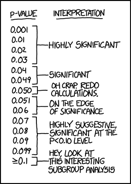
Source: https://xkcd.com/1478/

Preliminaries: The Problems with P-Value

• Adapting to this reverence to the 0.05, some researchers make small adjustments to their analysis when a p-value is slightly above 0.05 in order to try and push it below that threshold artificially. This practice is called p-hacking.

• So, we have an unintuitive, but very general, statistical method that gets overused by one group and reviled by another. These two groups aren’t mutually exclusive.

• The general-purpose feature is p-values is fantastic though, it’s hard to beat a p-value for appropriateness in varied situations. p-values aren’t bad, they’re just misunderstood. They’re also not alone.

Preliminaries: Confidence intervals

• Confidence intervals are ranges that are assumed to contain the true parameter value somewhere within them with a given probability. In many cases confidence intervals are computed alongside p-value by default.

The image on the next slide is by FRuDIxAFLG - Own work, CC BY-SA 4.0, https://commons.wikimedia.org/w/index.php?curid=114452600

Preliminaries: Confidence intervals

Preliminaries: Confidence intervals

• A hypothesis test can be conducted by checking if the confidence interval includes the null hypothesis value for the parameter.

• If we were looking for a difference between two means the null hypothesis would be that the mean is 0 and we would check if the confidence interval includes 0.

• If we were looking for a difference in odds we could get a confidence interval of the odds ratio and see if that includes 1.

Preliminaries: Confidence intervals

Two big advantages to confidence intervals over p-values:

• First, they explicitly state the parameter being estimated. If we’re estimating a difference of means, the confidence interval will also be measured in terms of a difference. If we’re estimating a slope effect in a linear regression model, the confidence interval will give the probable bounds of that slope effect.

• The other advantage is that confidence intervals imply the magnitude of the effect. Not only can we see if a slope or difference is plausibly zero given the data, but we can get a sense of how far from zero the plausible values reach.

Preliminaries: Confidence intervals

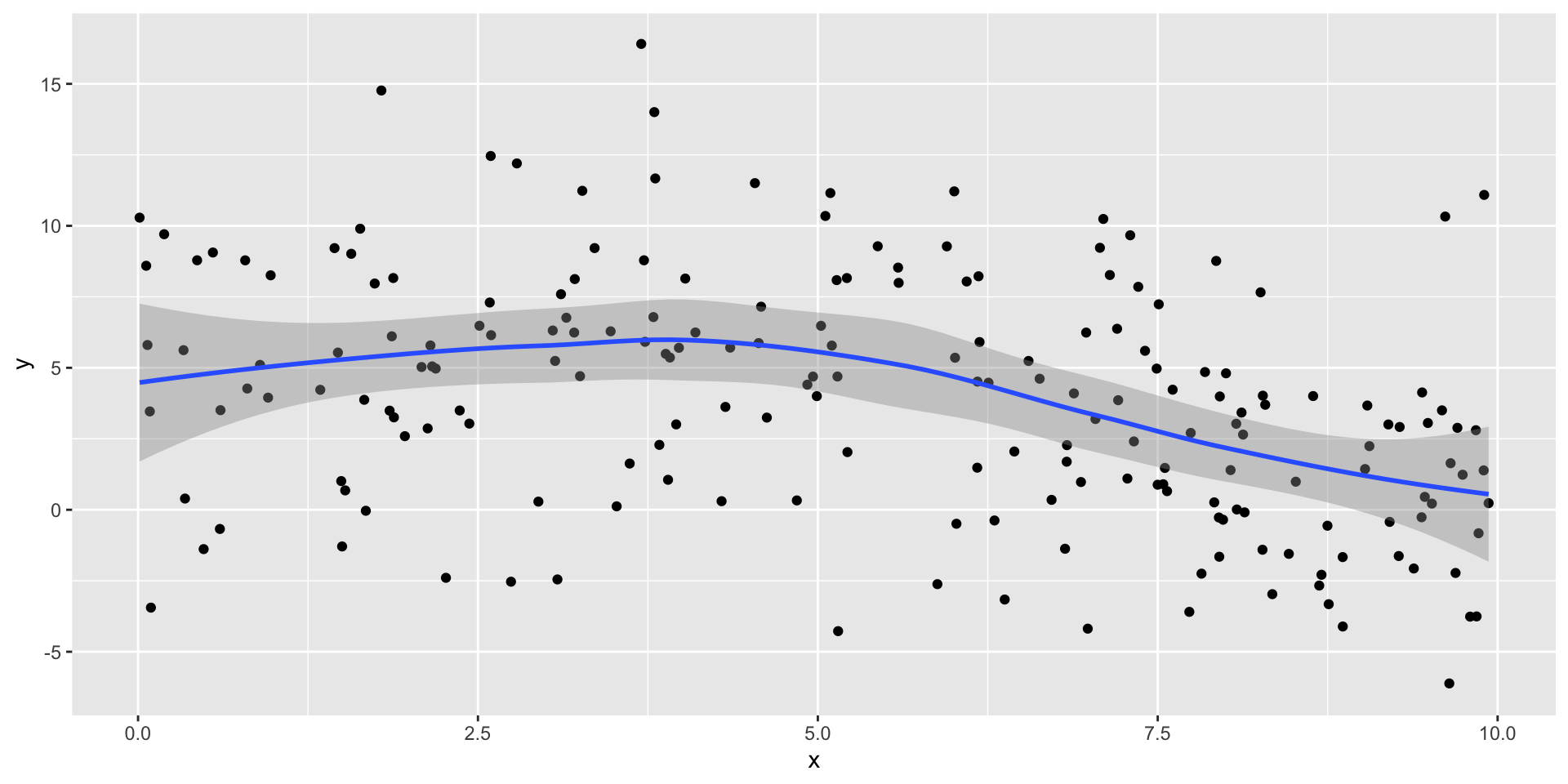
Furthermore, confidence intervals expand nicely into two-dimensional situations with confidence bands.

There are also Bayesian analogues called credible intervals and credible regions, which have a similar end results to confidence intervals / regions, but different mathematical interpretations.

Preliminaries: Confidence intervals

What is Magnitude Based Inference?

• Magnitude based inference (MBI) operates a lot like confidence intervals except that it also incorporates information about biologically or clinically significant effects.

• Magnitude based inference requires a confidence interval (generated in the usual ways) and two researcher-defined thresholds: one above and one below the null hypothesis value.

• MBI was developed for physiology and medicine, so these thresholds are usually referred to as the beneficial and detrimental thresholds, respectively.

What is Magnitude Based Inference?

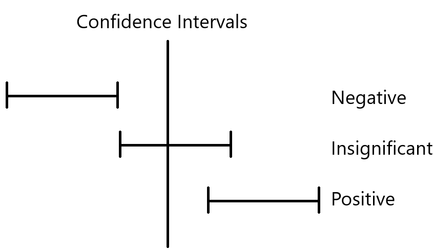
If we only had a null hypothesis value and a confidence interval we could make one of three inferences based on this information:

1. The parameter being estimated is less than the null hypothesis value

2. Is more than the null hypothesis value,

3. or it is uncertain.

These correspond to the confidence interval being entirely below the null hypothesis value, entirely above the null hypothesis value, and straddling the value respectively.

What is Magnitude Based Inference?

What is Magnitude Based Inference?

With these two additional thresholds, we can make a greater range of inferences. For example,

• If a confidence interval is entirely beyond the beneficial threshold, then we can say with some confidence is beneficial.

• If the confidence interval is entirely above the null hypothesis value, but includes the beneficial threshold, we can say with confidence that the effect is real and non-detrimental, and that it may be beneficial.

What is Magnitude Based Inference?

• If a confidence interval includes the null hypothesis value but no other threshold, we can say with some confidence that the effect is trivial. In other words, we don’t know what the value is but we’re reasonably sure that it isn’t large enough to matter.

What is Magnitude Based Inference?

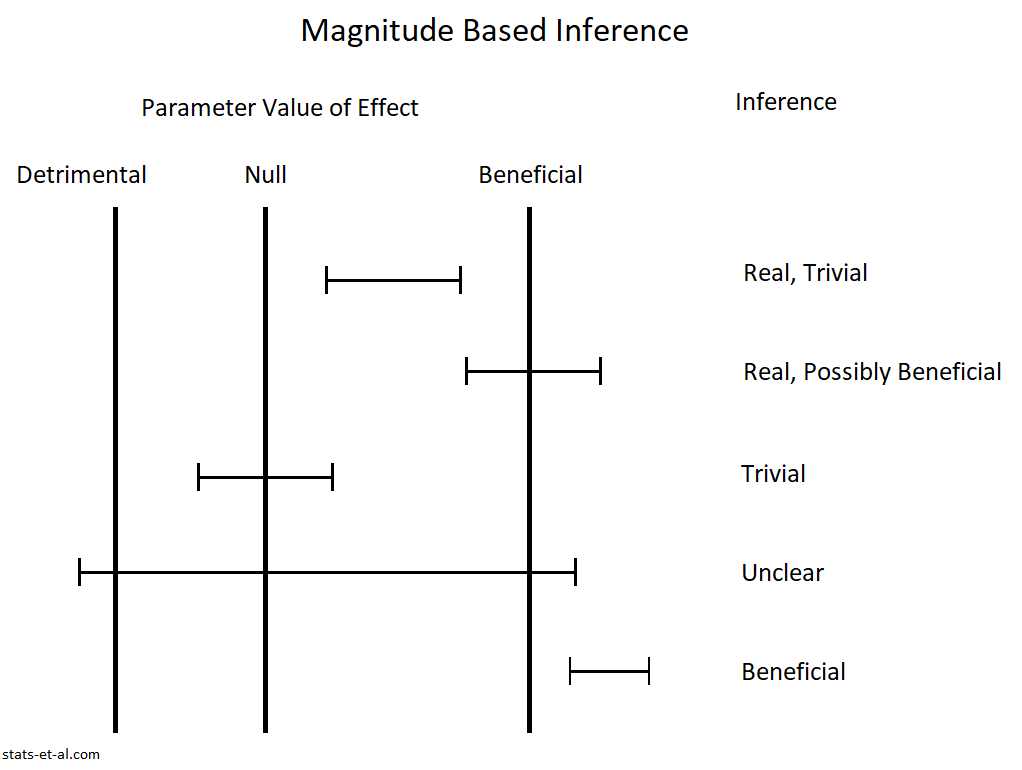
(See also: https://doi.org/10.1371/journal.pone.0235318.g002)

What is Magnitude Based Inference?

• MBI offers much greater insight than a p-value or a confidence interval alone, but it does require some additional expertise from outside of statistics in order to determine what is a minimum beneficial effect or a minimum detrimental effect.

• Sometimes thresholds involve guesswork, and often involve research discretion, so it also opens up a new avenue for p-hacking and abuse.

• However, as long as the thresholds are transparent, it’s easy to readers to check work for themselves.

What is the PROBLEM with MBI?

To quote the entire abstract of sportRxiv preprint at “Magnitude Based Inference in Relation to One-sided Hypotheses Testing Procedures” by Janet Aisbett, Daniël Lakens, and Kristin Sainani (My responses in bold)

Magnitude based inference (MBI) was widely adopted by sport science researchers as an alternative to null hypothesis significance tests.

• It has been criticized for lacking a theoretical framework, mixing Bayesian and frequentist thinking, so, like, all of data science?

…continued

What is the PROBLEM with MBI?

• and encouraging researchers to run small studies with high Type 1 error rates. valid, and that’s a big problem

• MBI terminology describes the position of confidence intervals in relation to smallest meaningful effect sizes. We show these positions correspond to combinations of one-sided tests of hypotheses about the presence or absence of meaningful effects, and formally describe MBI as a multiple decision procedure. Something like testing both \(\mu > 5\) and \(\mu < -5\) at the same time, valid

…continued

What is the PROBLEM with MBI?

…

• MBI terminology operates as if tests are conducted at multiple alpha levels. We illustrate how error rates can be controlled by limiting each one-sided hypothesis test to a single alpha level. That would be a good theoretical improvement

…continued

What is the PROBLEM with MBI?

…

To provide transparent error control in a Neyman-Pearson framework and encourage the use of standard statistical software, we recommend replacing MBI with one-sided tests against smallest meaningful effects, or pairs of such tests as in equivalence testing. Let’s explore this further.

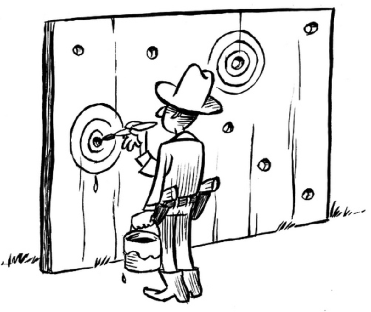
Researchers should pre-specify their hypotheses and alpha levels, perform a priori sample size calculations, and justify all assumptions. This is a lot of pre-registration of clinical studies, it’s useful for showing that you’re not committing the ‘painted bullseye fallacy’

Our recommendations show researchers what tests to use and how to design and report their statistical analyses to accord with standard frequentist practice. Great!

What is the PROBLEM with MBI?

Side note on the painted bullseye fallacy:

Pool games like billiards often require you to call the ball and the pocket before you hit the cue ball. That way all players know whether or not the ball you sunk was in fact the ball you meant to sink.

Likewise, pre-registration of clinical studies is where the background, experimental design, and hypotheses to be tests of a study are published somewhere (like a journal, such as Metapsychology) BEFORE the data are collected, so that it impossible (or much harder) to claim that a hypothesis was tested that happened to match what showed up as significant.

What is the PROBLEM with MBI?

Equivalence

We’ll come back to the problems with MBI, but let’s introduce some alternatives first.

Let’s start with the equivalence test, where we’re looking for evidence that one thing is equivalent to another. I.E.:

• Showing that a treatment does NOT produce a particular side effect by changing some parameter we don’t want to change. For example, we do NOT want a new nutritional supplement to raise OR lower blood pressure.

• Showing that a particular exercise or drill is waste of time.

• Showing that a particular auxilliary variable has no effect on player performance.

Equivalence

See also: “Chapter 09: Equivalence Testing and Interval Hypotheses” of the online book Improving Your Statistical Inferences by Daniël Lakens.

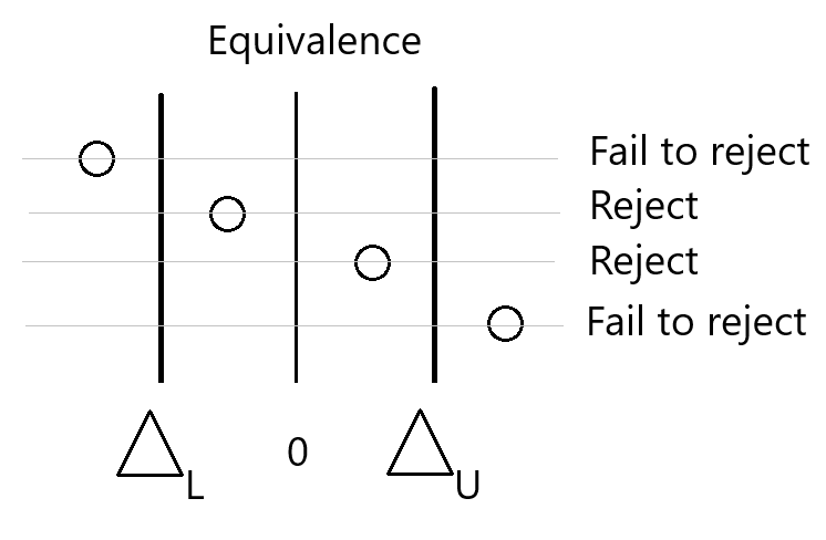
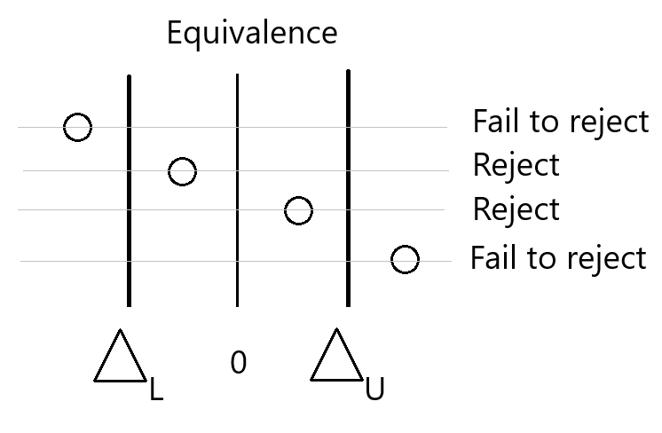
An equivalence test is like an inverted null hypothesis test. We need to show that something is sufficiently CLOSE to zero to reject the null that it isn’t.

This involves determining beforehand what a ‘clinically significant’ effect size is, and from that determining a \(\Delta_L\) and \(\Delta_U\) for the lower and upper bounds of what an equivalent effect size is.

Equivalence

Equivalence Test

To be clear, we’re talking about where the TRUE effect size is, not where the estimated effect size is and not where an interval that may capture the true effect size is.

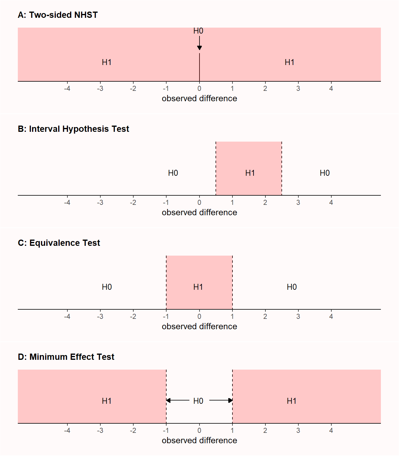
For comparison, the usual two-sided null hypothesis significance test (NHST) suggests that you take \(H_1\) (and reject \(H_0\)) if there is sufficient evidence that the true difference is anything other than zero.

Equivalence Test

From: https://lakens.github.io/statistical_inferences/09-equivalencetest_files/figure-html/fig-intervaltest-1.png

Equivalence

From “Equivalence Testing and Interval Hypotheses”

Equivalence tests are a specific implementation of interval hypothesis tests, where instead of testing against a null hypothesis of no effect (that is, an effect size of 0; nil null hypothesis), an effect is tested against a null hypothesis that represents a range of non-zero effect sizes (non-nil null hypothesis).

Aside: Minimum Effect Test

From “Equivalence Testing and Interval Hypotheses”

When an equivalence test is reversed, a researcher designs a study to reject effects less extreme than a smallest effect size of interest, it is called a minimum effect test (Murphy & Myors, 1999).

A researcher might not just be interested in rejecting an effect of 0 (as in a null hypothesis significance test) but in rejecting a range of effects that are too small to be meaningful.

Aside: Minimum Effect Test

All else [being] equal, a study designed to have high power for a minimum effect requires more observations than if the goal had been to reject an effect of zero. As the confidence interval needs to reject a value that is closer to the observed effect size (e.g., 0.1 instead of 0) it needs to be more narrow, which requires more observations.

One benefit of a minimum effect test compared to a null hypothesis test is that there is no distinction between statistical significance and practical significance. As the test value is chosen to represent the minimum effect of interest, whenever it is rejected, the effect is both statistically and practically significant (Murphy et al., 2014).

How to do an equivalence test

An equivalence test can’t be done with a single two-sided hypothesis test. Instead, we employ two one-sided tests (TOST). The formulae should be familiar:

\[\begin{align} t_L = \frac{\mathrm{(Observed\ Mean\ Diff) - (Hypothesis\ Cutoff)} }{\mathrm{SE(Mean\ Diff)}} = \\ \frac{(\bar y_1 - \bar y_2) - \Delta_L}{\sqrt{\frac{\sigma_1^2}{n_1} + \frac{\sigma_2^2}{n_2}}} \end{align}\]

How to do an equivalence test

and

\[\begin{align} t_U = \frac{\mathrm{(Observed\ Mean\ Diff) - (Hypothesis\ Cutoff)} }{\mathrm{SE(Mean\ Diff)}} = \\ \frac{(\bar y_1 - \bar y_2) - \Delta_U}{\sqrt{\frac{\sigma_1^2}{n_1} + \frac{\sigma_2^2}{n_2}}} \end{align}\]

where \(\sigma_{Pooled}\) is the usual pooled standard deviation of two groups.

How to do an equivalence test

As an example, consider:

Variable	Control	Fatigued
Mean	4.55	4.87
SD	1.05	1.12
n	15	15
Bound	Lower	Upper
Effect	-0.5	+0.5

How to do an equivalence test

res <- TOSTER::tsum_TOST(m1 = 4.55, m2 = 4.87, 
                         sd1 = 1.05, sd2 = 1.11,
                          n1 = 15, n2 = 15, 
                         low_eqbound = -0.5, high_eqbound = 0.5)

How to do an equivalence test

MET stands for “Minimum Effect Test”

plot(res, type = "tnull")

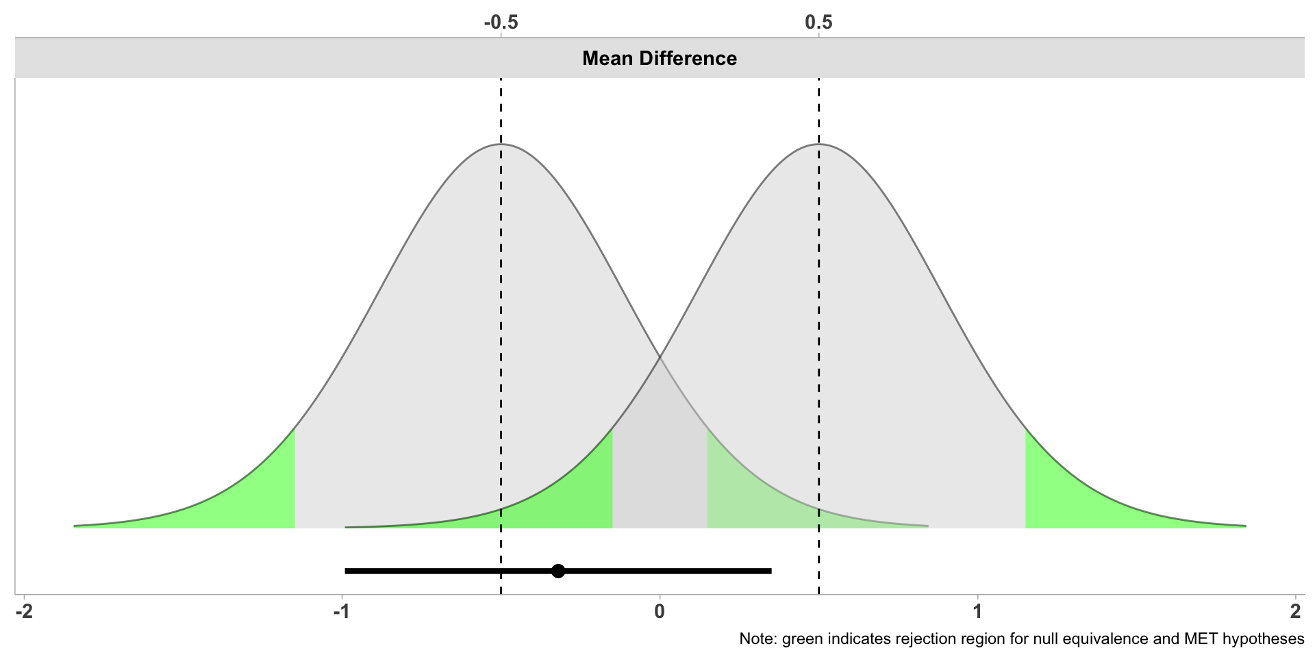
How to do an equivalence test

Another example:

Variable	Control	Fatigued
Mean	22.55	4.87
SD	5.05	1.12
n	30	15
Bound	Lower	Upper
Effect	-0.5	+0.5

How to do an equivalence test

res <- TOSTER::tsum_TOST(m1 = 22.55, m2 = 4.87, 
                         sd1 = 5.05, sd2 = 1.11,
                          n1 = 30, n2 = 15, 
                         low_eqbound = -0.5, high_eqbound = 0.5)

How to do an equivalence test

plot(res, type = "tnull")

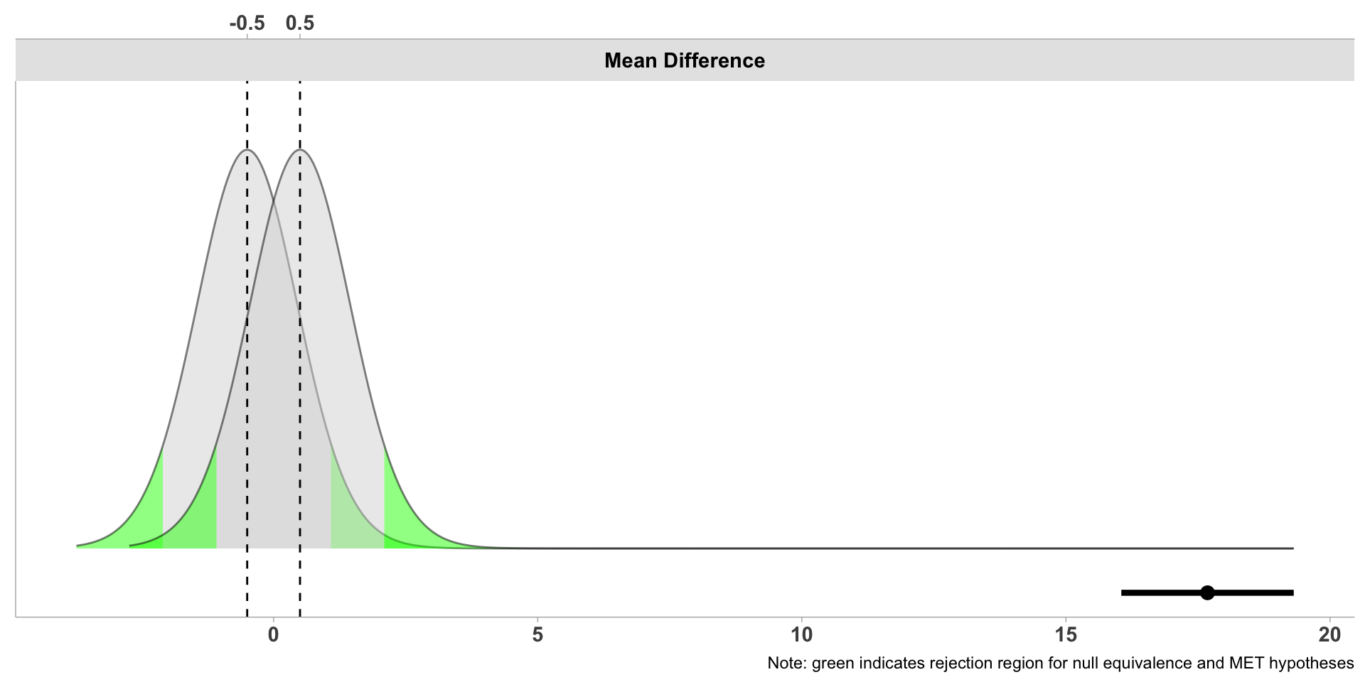
How to do an equivalence test

Notice how the conclusion is not to reject the null for the TOST? Because our confidence interval does not include both bounds.

res

How to do an equivalence test

Welch Two Sample t-test

The equivalence test was non-significant, t(34.21) = 17.794, p = 1e+00
The null hypothesis test was significant, t(34.21) = 18.311, p = 2.97e-19
NHST: reject null significance hypothesis that the effect is equal to zero 
TOST: don't reject null equivalence hypothesis

TOST Results 
               t    df p.value
t-test     18.31 34.21 < 0.001
TOST Lower 18.83 34.21 < 0.001
TOST Upper 17.79 34.21       1

Effect Sizes 
               Estimate     SE               C.I. Conf. Level
Raw               17.68 0.9655 [16.0477, 19.3123]         0.9
Hedges's g(av)     4.72 0.6509    [3.642, 5.7607]         0.9
Note: SMD confidence intervals are an approximation. See vignette("SMD_calcs").

How to do an equivalence test

One more example:

Variable	Control	Fatigued
Mean	4.55	4.87
SD	1.05	1.12
n	200	200
Bound	Lower	Upper
Effect	-1.25	+0.5

How to do an equivalence test

plot(res, type = "tnull")

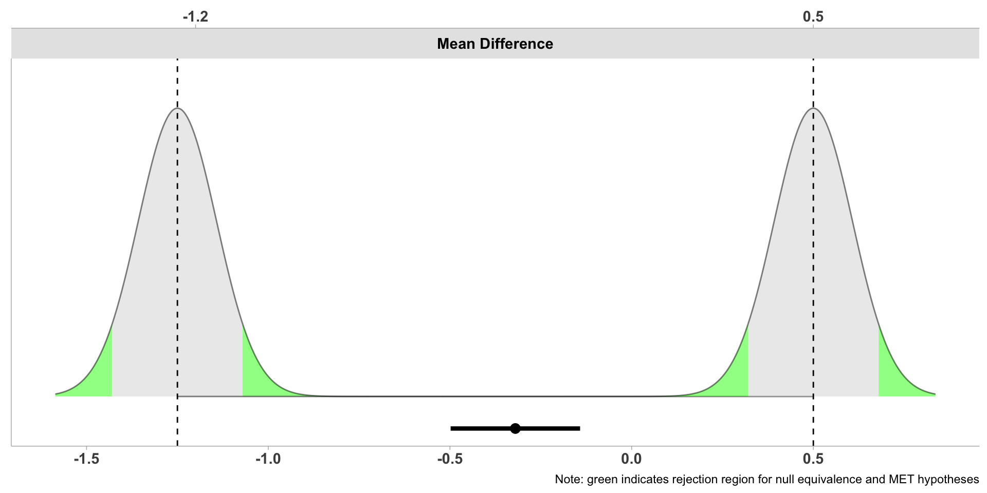
How to do an equivalence test

Final example:

Variable	Control	Fatigued
Mean	4.55	4.87
SD	1.05	1.12
n	10	10
Bound	Lower	Upper
Effect	-0.5	+0.5

How to do an equivalence test

res <- TOSTER::tsum_TOST(m1 = 4.55, m2 = 4.87, 
                         sd1 = 1.05, sd2 = 1.11,
                          n1 = 10, n2 = 10, 
                         low_eqbound = -0.5, high_eqbound = 0.5)

plot(res, type = "tnull")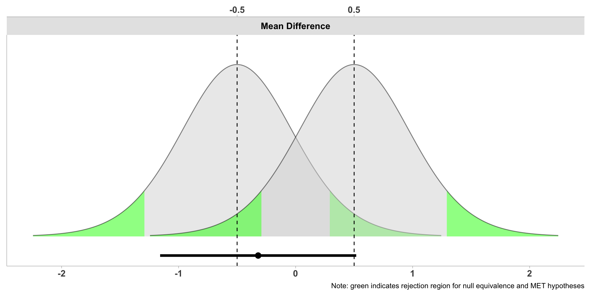

How to do an equivalence test

Notice how the confidence interval does NOT include zero, so the NHST response is to reject AND

Also the TOST of equivalence is to reject, because the confidence interval is entirely within the bounds.

How to do an equivalence test

res

Welch Two Sample t-test

The equivalence test was non-significant, t(34.21) = 17.794, p = 1e+00
The null hypothesis test was significant, t(34.21) = 18.311, p = 2.97e-19
NHST: reject null significance hypothesis that the effect is equal to zero 
TOST: don't reject null equivalence hypothesis

TOST Results 
               t    df p.value
t-test     18.31 34.21 < 0.001
TOST Lower 18.83 34.21 < 0.001
TOST Upper 17.79 34.21       1

Effect Sizes 
               Estimate     SE               C.I. Conf. Level
Raw               17.68 0.9655 [16.0477, 19.3123]         0.9
Hedges's g(av)     4.72 0.6509    [3.642, 5.7607]         0.9
Note: SMD confidence intervals are an approximation. See vignette("SMD_calcs").

Aside: Non-inferiority

From “Equivalence Testing and Interval Hypotheses”

A final variation of a one-sided non-nil null hypothesis test is known as a test for non-inferiority, which examines if an effect is larger than the lower bound of an equivalence range. Such a test is for example performed when a novel intervention should not be noticeably worse than an existing intervention, but it can be a tiny bit worse.

Aside: Non-inferiority

Examples include:

• Checking if a cheaper, faster, or less intensive training regimen produces results that are not inferior to the current standard of care, thereby freeing up resources to focus on other aspects of performance.

• Checking if a particular procedure is not harmful to performance. To clarify, wearing something for telemetrics or biometrics might be valuable for future testing, but if the wearable gets in the way during the sport it won’t be worn.

Aside: Non-Inferiority

https://pmc.ncbi.nlm.nih.gov/articles/PMC7734976/table/T1/

Setting delta-L and delta-U

From “Equivalence Testing and Interval Hypotheses”

To perform an equivalence test we need to specify which observed values are too small to be meaningful. … This requires that we specify the smallest effect size of interest (SESOI).

Setting delta-L and delta-U

From “Equivalence Testing and Interval Hypotheses”

Specifying a SESOI based on theory

(What does what we know already tell us about the SESOI?)

One example of a theoretically predicted smallest effect size of interest can be found in the study by Burriss et al. (2015), who examined whether women displayed increased redness in the face during the fertile phase of their ovulatory cycle.

…. (how can it be a signal of fertility if it can’t be noticed?)

Because the just-noticeable difference in redness of the skin can be measured, it was possible to establish a theoretically motivated SESOI.

Setting delta-L and delta-U

Anchor based methods to set a SESOI

(What do people implicitly tell us is the least meaningful difference?)

Measurements are collected at two time points (e.g., a quality of life measure before and after treatment). At the second time point, an independent measure (the anchor) is used to determine if individuals show no change

….

asked to answer the anchor question, and indicate if they subjectively feel the same, better, or worse at time point 2 compared to time point 1.

MBI in R, the mbir package.

Magnitude Based Inference in R and SAS - Using equivalence, non-inferiority, and minimal effects testing https://aaroncaldwell.us/blog/MBI/2020-05-04-magnitude-based-inference-in-r-and-sas.html

This is from the author of the mbir package, discussing what he did to adapt MBI to address these concerns. He demonstrates it in some three-sample cases.

Additional References

• My original hamfisted attempt at MBI

• Replacing Statistical Significance and Non-Significance with Better Approaches to Sampling Uncertainty

• “Can we trust “Magnitude-based inference?”

Final Items

• Course evaluations! https://perceptions.uwaterloo.ca

  • Feel free to write a novel, we’ll read all of the comments

  • This will be helpful for future classes, especially because this one technically doesn’t exist

Next Up

• Final Project due Monday, August 11 at 11:59 PM
• Check out LEARN for the office hours schedule