Lecture 4

2025-06-02

Case Study: Plus/Minus Modeling

Motivation

• We want to understand an individual’s contribution towards overall group output.
  • Applications to industry, sports, and economic inputs
• A lot of questions in sport can be framed as a constrained optimization problem where we try to maximize an objective function given scarcity in resources, which in this case is “talent”.

Motivation

• When a coach decides how to construct a lineup, they must consider how each player contributes to team success. This is why it is imperative to create metrics that are able to appropriately quantify player contribution.
• There are multiple angles that we can use for credit assignment between players, including their actions, physical attributes, intentions, and movement patterns.
  • Today’s talk will focus on the least granular aspect of player contribution modeling - player presence.

Metric Creation

When aspiring to create metrics for a sport, or any field for that matter, we have to constantly remind ourselves that what we are doing must be done for the advancement of the sport. I follow 3 general principles:

1. Practical Significance
2. Technical Contribution
3. Data Constraints

1. Practical Significance

• This is the most important consideration, with which we can envision the kind of impact our metric will have on how the game is played and coached.

• This requires copious amounts of subject matter awareness to identify where the current literature stands and have firsthand accounts from coaches and players about the different areas in the sport that are still yet to be “solved”.

• Tied in closely with the impact is the way that the finding can be implemented in a designated training environment.

2. Technical Contribution

• This can take many forms, such as new metrics, strategies and tactics, and a comprehensive mathematical foundation from which insights are generated.

• We are at a point in sports analytics where we can take full advantage of the high quality data being tracked in so many leagues to apply complex mathematical functions and models with robust validation strategies.

• Many recent sports analytics research papers have been published in high quality theoretical and applied journals, a testament to their mathematical rigor.

It comes as no surprise that many recent sports analytics research papers have been published in journals such as the Annals of Applied Statistics, a testament to their mathematical rigor.

3. Data Constraints

For both implementation purposes and insights, data constraints must be taken into account so that we can identify areas to invest in new technology, while ensuring that our current approaches aren’t lost.

Meta-Analytics

• We can use a set of “meta-metrics” called meta-analytics (Franks et al, 2016) to evaluate the quality of metrics.
• Under this framework, we consider three main attributions of each metric:
  • Stability: How well does the metric measure itself over time?
  • Discrimination: How well does the metric differentiate between players?
  • Independence: How much new information does the metric give compared to existing metrics?

Meta-Analytics

• For example, in the NBA metrics like Win Shares and Value over Replacement Player (VORP) are more reliable (have greater stability) than rate-based statistics like eFG%, but actually have a weaker signal (less independence) than these metrics.
• Prof. Wong will deliver a more detailed lecture on meta-analytics later this semester.

Modeling Player Contribution via Player Presence

• The first level of player contribution Modeling is addressed by asking the following question: “How can we quantify the magnitude of contribution via knowledge of player identity?”
  • This inspires player presence models.
• Player presence models decompose team success and divide credit from these outcomes between individual players active at the time of that outcome.

Modeling Player Contribution via Player Presence

• These methods aim to capture player impact without explicitly specifying the forms that they take, which allows us to account for latent contributions such as teamwork effects and other player intangibles.
• This also helps quantify the influence that players have on the decision making of their opponents and teammates.
• Typical measures for team success used as outcomes in player presence models are wins, points, and their derivative probabilities and scaled differentials.

Worked Example

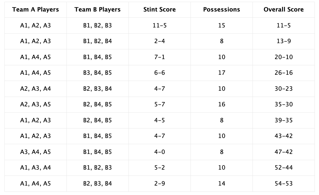
Consider a toy 3x3 basketball example derived from Squared2020 where each team has 5 players. The final score is 54 - 53 for team A and the point-differential is as follows:

Level 1: Traditional Plus/Minus

• Plus/Minus is a simple counting statistics that for each player takes the difference of the points scored and points conceded by their team while they are on the court.
• Plus/Minus originated in the National Hockey League (NHL) in the 1950’s and 60’s and has since been adopted extensively in basketball, soccer, and other leagues around the world.

Level 1: Traditional Plus/Minus

Using the previous example, the plus/minus for each player would be as follows:

Team A	Team B
A1: +2	B1: -14
A2: -5	B2: +6
A3: +2	B3: +3
A4: +3	B4: +6
A5: +1	B5: -4

What are some of the benefits and drawbacks of raw plus/minus?

Raw Plus/Minus: Discussion

• Benefits:
  • High interpretability
  • Linear scaling
  • Easy data collection
• Drawbacks:
  • Low discriminatory power: difficult to distinguish between players
  • Teammate and opponent agnostic
  • Ignores player roles and playing time adjustments

• Poor players on good teams are overrated, while good players on poor teams are underrated.

Level 2: Adjusted Plus/Minus (APM): The Intuition

• Adjusted Plus/Minus (APM) was introduced Dan Rosenbaum in 2004 to extend Plus/Minus using a system of linear equations to represent active player on the court.
• Here, we take the score differential at each game stint \(s\), convert it to a \(\text{per}-100\) possessions basis, and regress the active players on it.
• Therefore, an active player \(X_i\) on the home team (team A) is given a coefficient of \(+1\), while an active player on the visiting team (team B) is given a coefficient of \(-1\).

Level 2: Adjusted Plus/Minus (APM): The Intuition

• Players on either side who are inactive during a particular stint are given a value of \(0\).
• Since the score differential and player coefficients are given from the perspective of the home team, the intercept term \(\beta_0\) serves to capture home court advantage, and the remaining \(\beta_i\)’s are used as estimates for player contribution.

Level 2: Adjusted Plus/Minus (APM): The Intuition

\[Y_1 = \beta_0 + \beta_1A_{1,1} + \beta_2A_{2,1} + \beta_3A_{3,1} + \beta_4A_{4,1} + \beta_5A_{5,1} +\] \[\beta_6B_{1,1}+ \beta_7B_{2,1} + \beta_8B_{3, 1} + \beta_9B_{4,1} + \beta_{10}B_{5,1}\] \(\vdots\)

\[Y_s = \beta_0 + \beta_1A_{1,s} + \beta_2A_{2,s} + \beta_3A_{3,s} + \beta_4A_{4,s} + \beta_5A_{5,s} +\] \[\beta_6B_{1,s}+ \beta_7B_{2,s} + \beta_8B_{3, s} + \beta_9B_{4,s} + \beta_{10}B_{5,s}\]

Level 2: Adjusted Plus/Minus (APM): The Intuition

• Additional contextual game variables serving as proxies for leverage were also used in the model, improving APM’s ability to distinguish player contribution from situational factors.

• To help ensure that the matrix used in the OLS estimate is invertible, Rosenbaum removes players who have extremely low usage rates from the data set.

Level 2: Adjusted Plus/Minus (APM): The Intuition

• For example, the first stint between player A1, A2, A3 vs. B1, B2, B3 would be calculated as +6 over 15 possessions = +40 over 100 possessions, with nonzero coefficients for the active players and zeroes otherwise.

\[40 = \beta_0 + \beta_1*1 + \beta_2*1 + \beta_3*1 + \beta_4*0 + \beta_5*0 -\] \[\beta_6*1-\beta_7*1-\beta_8*1-\beta_9*0-\beta_{10}*0\]

What are some of the benefits and drawbacks of adjusted plus/minus?

Adjusted Plus/Minus: Discussion

• Benefits:
  • Improved discrimination
  • Very interpretable: The relative expected point differential in contribution with respect to their replacement.
• Drawbacks
  • Exploding Residuals
  • Multicollinearity
  • Overfitting

Level 3: Regularized Adjusted Plus/Minus (RAPM): The Intuition

• To address the issue of multicollinearity, Sill (2010) applied a Bayesian technique called Regularization.
• This is a penalized regression model where bias is introduced to combat overfitting and improve accuracy.
• More commonly known as ridge regression, the new estimates of the parameters \(\beta_i\) are found as:

\(\boldsymbol{\beta} = \arg \min_{\boldsymbol{\beta}} \sum_{i=1}^{N}[y_i-\boldsymbol{X\beta}]^2 + \lambda||\boldsymbol{\beta}||_2^2\)

• With the 3x3 example, the coefficients shrink to much more reasonable levels and B4 had the largest value.

What are some of the benefits and drawbacks of regularized adjusted plus/minus?

RAPM: Discussion

• Benefits:
  • Stability: Required less data and no removal of players since we can guarantee an invertible matrix
  • Discrimination: Finally revealed the value of underrated players such as Shane Battier
• Drawbacks:
  • Interpretability: All interpretation must be made relative to the chosen lambda value
  • Subjectivity in formulation

Level 4: Plus/Minus Extensions

• Many extensions to plus/minus algorithms have been implemented in basketball, such as EPM and RAPTOR.

• Example: Box Plus/Minus 2.0 (BPM) (Myers, 2020)

  • BPM was created to combine the benefits of player presence and player action frameworks, while remaining accessible to many levels of competitive sport due to its reliance on match summary statistics.
  • The base model regresses a player’s RAPM on their match summary statistics, making adjustments for overall team quality, usage rates, and player roles.

Level 4: Plus/Minus Extensions

• Points Above Average Per Set (PAAPS) (Fellingham, 2022) uses a baseline RAPM model regressed on player contacts instead of player presence for metrics in volleyball.

  • This adds more context to contribution in terms of the quantity of contacts and how they influence team possession, but stills fails to discriminate between different contact types and how credit is distributed.

• In ice hockey, Thomas et al, 2013 make analogs to offensive and defensive ratings using competing process hazard function models with penalized estimation.

• This adds more context to contribution in terms of the quantity of contacts and how they influence team possession, but it stills fails to discriminate between different contact types and how credit is distributed between players.

Level 4: Plus/Minus Extensions

• In volleyball, Hass & Craig, 2018 made several plus/minus models in volleyball. Instead of combining sequences of points by player stints as done in basketball, Hass considered each point as its own independent entity.

• Therefore we are now predicting point-win probability, and at a high level the model can be understood as a logistic regression of Win probability ∼ contextual variables + player variables.

• A comprehensive review of plus/minus models across different sports was conducted by Hvattum in 2019.

Conclusion - Custom Plus/Minus Models

Now that we’ve covered the methodology and existing examples of plus/minus models, let’s brainstorm how we’d make our own!

• Would plus/minus work better in higher scoring or lower scoring sports?
• Where can you find play-by-play data? Are there additional data sources that you could leverage?
• What other covariates could you include in your plus/minus model?

Conclusion - Custom Plus/Minus Models

• What types of penalties could we use?
  • L2 is the standard for ridge regression, but LASSO, which sums the absolute value of the coefficients instead of squaring them could also be used
  • Bayesian formulations (using a Gaussian or Laplacian prior) can also be considered.
  • Potential to use an elastic net, which is a hybrid between ridge and lasso penalties.

• which is able to flexibly shrink coefficients without meaningful impact on estimates while simultaneously maintaining the magnitudes of those that do matter.

Conclusion - Custom Plus/Minus Models

• What are other sports where plus/minus could be used?
• What are the underlying assumptions of RAPM and the math necessary to keep this accountable?
  • How do we account for aging curves?
• Code implementations:
  • 2017 NBA Data in R.
  • Tony El Habr: NBA RAPM in R
  • Kaggle: Calculating RAPM in Hockey using Python

Next Up

• Module 2: Introduction to Data Science
  • R4DS Chapters 23-29
  • P4DS: Chapters 25-31
• Assignment 4: Due June 9 @ 11 AM on Crowdmark