Lecture 5
2025-06-09
Case Study: An introduction to Elo ratings using NFL game outcomes
Dr. Ron Yurko - Carnegie Mellon University
Overview
Elo ratings are a popular approach for estimating player/team strength across different sports. A number of sports examples are maintained by sportswriter Neil Paine, as well as older versions featured in FiveThirtyEight.
These dynamic ratings are adjusted for opponent strength and can be used for historical comparisons, such as who is the greatest tennis player of all time?, and for predicting outcomes.
In this module you will learn the basics of Elo ratings in the context of measuring NFL team strength, walking through steps to implement and assess Elo ratings from scratch in R.
Learning Objectives
By the end of this module, you will be able to:
- Compute the expected outcome or predicted probability based on player/team ratings.
- Update ratings following the observed outcome of a match/game.
- Implement the complete Elo ratings framework in R for a full NFL season.
- Assess Elo rating predictions using Brier scores.
- Tune the update factor and other settings to yield more optimal predictions.
Intro and Data
The purpose of this module is to introduce the basics of Elo ratings in the context of measuring NFL team strengths.
We’ll use a subset of the NFL Game Outcomes dataset available on the SCORE Sports Data Repository, only considering games during the 2023-24 season.
Intro and Data
The following code chunk reads in the larger dataset and filters down to only include games during the 2023-24 season:
url: https://data.scorenetwork.org/data/nfl_mahomes_era_games.csv
Intro and Data
As indicated in the overview page for the larger dataset, each row in the dataset corresponds to a single game played during the 2023-24 season:
| season | game_id | game_type | week | home_team | away_team | home_score | away_score | game_outcome | score_diff |
|---|---|---|---|---|---|---|---|---|---|
| 2023 | 2023_01_DET_KC | REG | 1 | KC | DET | 20 | 21 | 0 | -1 |
| 2023 | 2023_01_CAR_ATL | REG | 1 | ATL | CAR | 24 | 10 | 1 | 14 |
| 2023 | 2023_01_HOU_BAL | REG | 1 | BAL | HOU | 25 | 9 | 1 | 16 |
| 2023 | 2023_01_CIN_CLE | REG | 1 | CLE | CIN | 24 | 3 | 1 | 21 |
| 2023 | 2023_01_JAX_IND | REG | 1 | IND | JAX | 21 | 31 | 0 | -10 |
| 2023 | 2023_01_TB_MIN | REG | 1 | MIN | TB | 17 | 20 | 0 | -3 |
Intro and Data
Note the game_type column indicates if the game was during the regular season (REG), or during the playoffs with the different values indicating the different playoff rounds:
The week column just increases in the correct order, which will be convenient for implementing Elo ratings over the course of the NFL season.
Background Information
Elo ratings were created by physicist Arpad Elo in the 1950s for rating chess players.
The point of the rating system is to compute ratings that could be used to estimate relative strength and predict game outcomes.
The main idea behind Elo ratings is to create an exchange in rating points between players (or teams) after a match.
Background Information
The simplest version of this system was constructed to be a zero-sum rating, such that the winner gains x points while the same number of x points are subtracted from the loser’s rating.
If the win was expected, the winner receives fewer points than if the win was unexpected (i.e., an upset) - where the expectation is set prior to the match.
This system results in a dynamic rating that is adjusted for opponent quality.
Method Details
We’re going to consider a simple version of Elo ratings in the context of measuring NFL team strength via a rating.
Let the rating for the home team be \(R_{\text{home}}\) and the away team rating be \(R_{\text{away}}\).
Then the expected score for the home team \(E_{\text{home}}\) is calculated as:
\[ E_{\text{home}} = \frac{1}{1+10^{\left(R_{\text{away}}-R_{\text{home}}\right) / 400}}, \]
Method Details
The expected score for the away team \(E_{\text{away}}\) is computed in a similar manner:
\[ E_{\text{away}} = \frac{1}{1+10^{\left(R_{\text{home}}-R_{\text{away}}\right) / 400}}. \]
These expected scores represent the probability of winning1, e.g., \(E_{\text{home}}\) represents the probability of winning for the home team.
Method Details
The choice of 10 and 400 in the denominator may appear arbitrary at first, but they correspond to:
- a logistic curve (thus bounded by 0 and 1) with base 10, and
- a scaling factor of 400 which can be tuned to yield better predictions (discussed in more detail on the next slide).
Method Details
A more general representation of the expected score would replace the choice of 10 with some constant (e.g., \(e\)) and replace 400 with a tune-able quantity \(d\).
For now though we will just use 10 and 400 since they are the original choices.
While the above quantities represent the expectation of a game between teams with ratings \(R_{\text{home}}\) and \(R_{\text{away}}\), we need a step to update the ratings after observing the game outcome.
Method Details
We update the ratings for the home team based on the observed score \(S_{\text{home}}\):
\[ R^{\text{new}}_{\text{home}} = R_{\text{home}} + K \cdot (S_{\text{home}} - E_{\text{home}}) \]
The observed score \(S_{\text{home}}\) is based on the game outcome such that,
- \(S_{\text{home}} = 1\) if the home team wins,
- \(S_{\text{home}} = 0.5\) if it is a tie, or
- \(S_{\text{home}} = 0\) if the home team loses.
Method Details
We compute the updated rating for the away team \(R^{\text{new}}_{\text{away}}\) in a similar manner, by replacing home team quantities with those for the away team.
The quantity \(K\) is known as the update factor, indicating the maximum number of Elo rating points a team gains from winning a single game (and how many points are subtracted if they lose).
This is a tuning parameter, which ideally should be selected to yield optimal predictive performance.
Thought Exercise #1
QUESTION: Given the above equation for \(R^{\text{new}}_{\text{home}}\), what do you think will happen as you increase \(K\)?
Does a single game cause a larger or smaller change on a team’s rating?
Likewise, what do you think will happen if you decrease \(K\)? What do you expect to observe?
Thought Exercise #1
ANSWER: The update factor \(K\) controls how sensitive the ratings should be to a single game outcome.
- A larger choice of \(K\) will lead to a larger change in a team’s rating following a single game, and likewise a smaller choice of \(K\) will lead to a smaller change in a team’s rating.
Although the details are beyond the scope of this module, there is a relationship between this Elo ratings update formula with stochastic gradient descent for logistic regression.
Worked Example
We’ll now proceed to implement Elo ratings for NFL teams during the 2023-24 season in R.
We will start by creating two helper functions to compute the expected scores and updated ratings after a game.
Calculate Expected Score
Based on the formulas for expected score, we write a function calc_expected_score that takes in as input a team_rating and opp_team_rating then returns the expected score for the team relative to the opp_team.
- For ease, our function uses the base 10 logistic curve and scaling factor of 400 as fixed quantities.
Calculate Expected Score Example
Using calc_expected_score, the expected score for a team with a rating of 1400 playing against an opposing team with a rating of 1600 is about 0.24, indicating that the team with a rating of 1400 has an estimated 24% chance of beating an opponent with a rating of 1600.
Calculate Updated Rating
Next, we complete the calc_new_rating function that takes in an initial team_rating, the observed_score and expected_score with respect to that team, along with a choice of the update_factor \(K\) to return the new rating.
- For now, we will just consider \(K = 20\) as the default choice.
Calculate Updated Rating Example
Using calc_expected_score and calc_new_rating together with \(K = 20\), the new rating for team that had an initial rating of 1300 but beat an opponent with a rating of 1700 is roughly 1318.
Since the maximum number of possible points is \(K = 20\), this is indicative of how beating a team with a rating of 1700 was relatively unexpected and nearly earned the team the maximum possible 20 points.
NFL Elo Ratings
Now with the basics, let’s move on to perform these calculations over the entire season, updating a table to include each team’s Elo rating following every game.
We can implement this using a for loop to proceed through each game in the nfl_games table, looking up each team’s previous ratings and performing the above calculations.
Prior to beginning this loop, we will set-up a table initializing each team with a rating of 1500.
This a naive approach since we likely have prior knowledge about each team’s strength before the start of the season, but we’ll discuss this in more detail at the end of the module.
NFL Elo Ratings
For now, we’ll use 1500 since it is a common choice for initializing Elo ratings. The code chunk below initializes this starting table of ratings beginning with an imaginary week 0:
NFL Elo Ratings
for (game_i in 1:nrow(nfl_games)) {

  # Grab the home and away teams in the current game:
  home_team <- nfl_games$home_team[game_i]
  away_team <- nfl_games$away_team[game_i]
  # What was the observed score by the home team?
  observed_home_score <- nfl_games$game_outcome[game_i]
  # Retain the week number for this game:
  game_week <- nfl_games$week[game_i]
NFL Elo Ratings
...
  # What was each team's rating from their latest game in the
  # current elo ratings table, starting with the home team:
  home_rating <- nfl_elo_ratings |>
    filter(team == home_team) |>
    # Sort in descending order
    arrange(desc(week)) |>
    # Grab the latest game
    slice(1) |>
    # Just return the elo rating
    pull(elo_rating)
  # Same thing for away team
  away_rating <- nfl_elo_ratings |>
    filter(team == away_team) |>
    arrange(desc(week)) |>
    slice(1) |>
    pull(elo_rating)
NFL Elo Ratings
...
  # Now get their new ratings, starting with the home team:
  new_home_rating <- calc_new_rating(home_rating, observed_home_score,
                                     calc_expected_score(home_rating,
                                                         away_rating))
  # And repeating for the away team using the opposite input as home team:
  new_away_rating <- calc_new_rating(away_rating, 1 - observed_home_score,
                                     calc_expected_score(away_rating,
                                                         home_rating))
  # Set up a table containing the updated ratings for each team
  updated_ratings <- tibble(team = c(home_team, away_team),
                        elo_rating = c(new_home_rating, new_away_rating),
                        # Store the week index of the game
                        week = rep(game_week, 2))
  # Add each teams new ratings to the current elo ratings table:
  nfl_elo_ratings <- nfl_elo_ratings |>
    bind_rows(updated_ratings)
}
NFL Elo Ratings
After we run the completed for loop, we can view and inspect the ratings in different ways.
For example, the following code chunk will return the final rating for each after the completion of the entire season of games:
nfl_elo_ratings |>
  group_by(team) |>
  # Since some teams make the playoffs, need to find the rating
  # for each team's final weeK:
  summarize(final_rating = elo_rating[which.max(week)]) |>
  # Sort in descending order of the rating so the best team is first:
  arrange(desc(final_rating)) %>% slice_head(n = 15) %>% gt()
NFL Elo Ratings
| team | final_rating |
|---|---|
| KC | 1575.945 |
| BAL | 1575.354 |
| SF | 1563.868 |
| DET | 1561.016 |
| BUF | 1546.537 |
| DAL | 1546.030 |
| CLE | 1532.056 |
| HOU | 1527.808 |
| MIA | 1525.271 |
| LA | 1523.254 |
| PHI | 1518.690 |
| PIT | 1517.095 |
| CIN | 1515.539 |
| GB | 1513.912 |
| TB | 1509.230 |
Change in Team Ratings Over Time
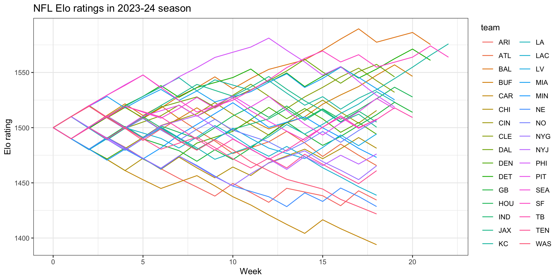
It is often helpful to visualize how the team ratings are changing over time. The following code creates a line for each team:
Change in Team Ratings Over Time
Change in Team Ratings Over Time
While we can observe ratings changing over the season for every team, this visualization is less than ideal.
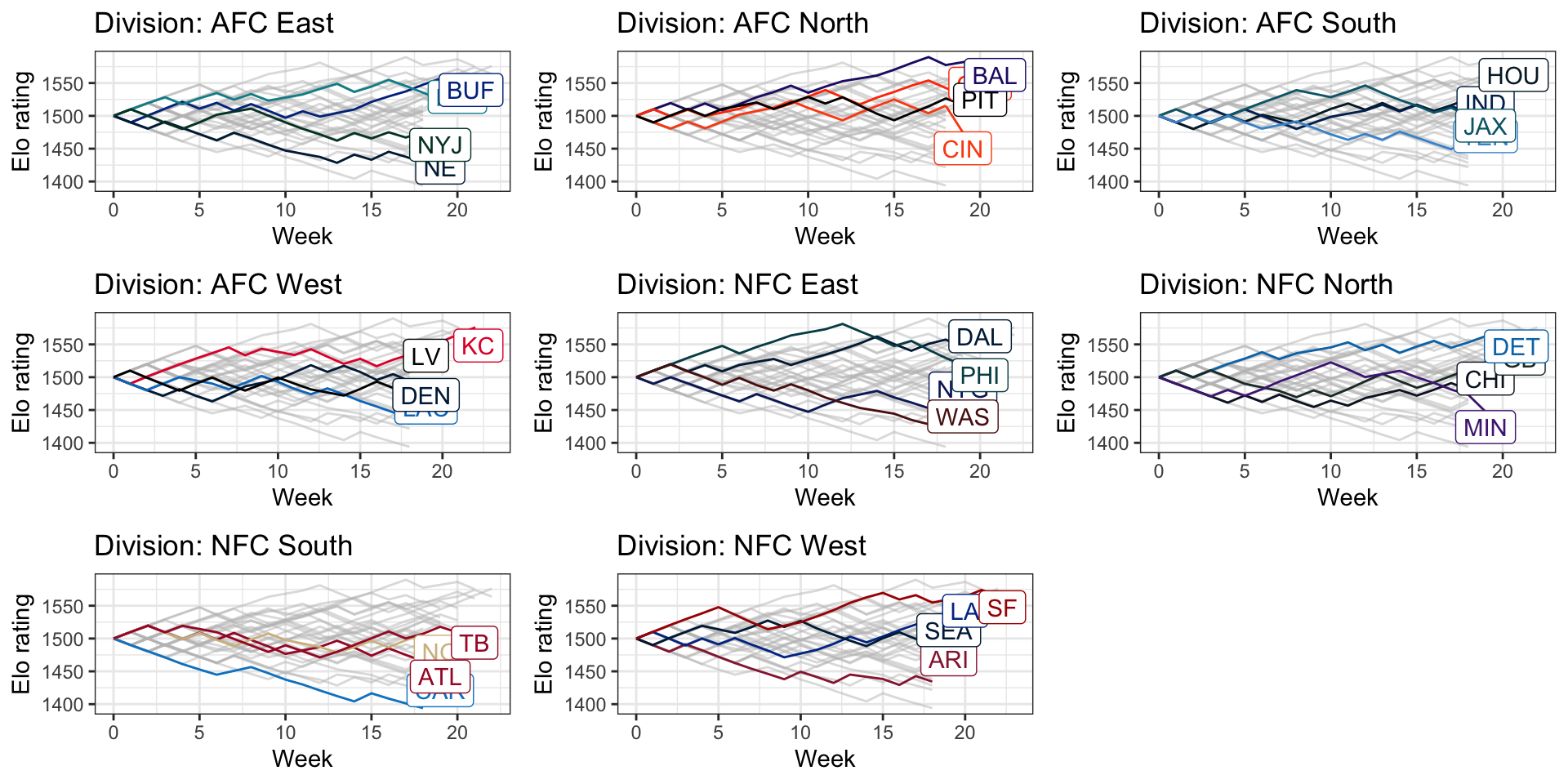
Instead one could take advantage of the team colors available using the load_teams function from the nflverse.
This is a little more involved, but here is example way to create a figure highlighting teams in each division separately (this requires installing the nflreadr, ggrepel, and cowplot packages:
Change in Team Ratings Over Time
library(nflreadr)
nfl_team_colors <- load_teams() |>
  dplyr::select(team_abbr, team_division, team_color)

# Create a dataset that has each team's final Elo rating
nfl_team_final <- nfl_elo_ratings |>
  group_by(team) |>
  summarize(week = max(week),
            elo_rating = elo_rating[which.max(week)],
            .groups = "drop") |>
  inner_join(nfl_team_colors, by = c("team" = "team_abbr")) |>
  arrange(desc(elo_rating))
Change in Team Ratings Over Time
...
library(ggrepel)
division_plots <-
  lapply(sort(unique(nfl_team_final$team_division)),
         function(nfl_division) {
             # Pull out the teams in the division
             division_teams <- nfl_team_final |>
               filter(team_division == nfl_division) |>
               mutate(team = fct_reorder(team, desc(elo_rating)))
             # Get the Elo ratings data just for these teams:
             division_data <- nfl_elo_ratings |>
               filter(team %in% division_teams$team) |>
               mutate(team = factor(team,
                              levels = levels(division_teams$team))) |>
               group_by(team) |>      # Make text labels for them:
               mutate(team_label = if_else(week == max(week),
                                           as.character(team),
                                           NA_character_)) |> ungroup()
Change in Team Ratings Over Time
...
         nfl_elo_ratings |>
           # Plot all of the other teams as gray lines:
           filter(!(team %in% division_teams$team)) |>
           ggplot(aes(x = week, y = elo_rating, group = team)) +
           geom_line(color = "gray", alpha = 0.5) +
           # But display the division teams with their colors:
           geom_line(data = division_data,
                     aes(x = week, y = elo_rating, group = team,
                         color = team)) +
           geom_label_repel(data = division_data,
                            aes(label = team_label,color = team),
                            nudge_x = 1, na.rm = TRUE, direction = "y") +
           scale_color_manual(values = division_teams$team_color,
                              guide = FALSE) + theme_bw() +
           labs(x = "Week", y = "Elo rating",
                title = paste0("Division: ", nfl_division))
         })
Change in Team Ratings Over Time
Assessing the Ratings
The result of the for loop from above provides us with a dataset that contains the rating for each team after every week. But how do we know if we can trust this approach for estimating team ratings?
We can assess the predictive performance of the Elo ratings based on the estimated probabilities for every game given the team’s ratings entering the game.
Missing Team Ratings
To demonstrate this, we will first need to fill in for missing weeks for teams due to bye weeks.
You can see in the output from the table counts below that during certain weeks there are fewer than 32 teams with ratings (this is not a concern in the values post week 18 since that corresponds to playoffs):
Missing Team Ratings
We fix this issue by iterating over each possible week, and fills in missing week ratings with the last available rating.
# First get a vector of the unique teams from the table:
nfl_teams <- unique(nfl_elo_ratings$team)

# Now iterate over the weeks and decide how to grab the team ratings
complete_nfl_elo_ratings <-
  map_dfr(unique(nfl_elo_ratings$week),
          function(week_i) {

            # How many teams have ratings in the week?
            covered_teams <- nfl_elo_ratings |>
              filter(week == week_i) |>
              pull(team) |>
              unique()
Missing Team Ratings
...
            if (length(nfl_teams) == length(covered_teams)) {
              # Just return the rows from the nfl_elo_ratings table:
              nfl_elo_ratings |>
                filter(week == week_i)

            } else {
              # Otherwise, we need to fill in the missing teams
              # 1. Get the latest ratings for every team before this week:
              latest_ratings <- nfl_elo_ratings |>
                filter(week < week_i) |>
                group_by(team) |>
                summarize(elo_rating = elo_rating[which.max(week)],
                          .groups = "drop") |>
                mutate(week = week_i)
Missing Team Ratings
...
              # Now gather the ratings for teams that are not missing this week:
              week_ratings <- nfl_elo_ratings |>
                filter(week == week_i)
              # Join together the missing ratings and return:
              week_ratings |>
                bind_rows(filter(latest_ratings,
                                 !(latest_ratings$team %in%
                                     week_ratings$team)))
            }
          })

# And this now fixes the previous problem:
table(complete_nfl_elo_ratings$week)
 0  1  2  3  4  5  6  7  8  9 10 11 12 13 14 15 16 17 18 19 20 21 22
32 32 32 32 32 32 32 32 32 32 32 32 32 32 32 32 32 32 32 32 32 32 32
Home and Away Elo Ratings
We now make two copies of the complete_nfl_elo_ratings table - one to use for home teams and another to use for away teams. The code chunk below initializes these copies and adds 1 to the week column to indicate which week to use team’s rating when predicting:
home_elo_ratings <- complete_nfl_elo_ratings |>
  mutate(week = week + 1) |>
  # Rename the team and elo_rating columns
  rename(home_team = team,
         home_elo_rating = elo_rating)

# And repeat for away teams:
away_elo_ratings <- complete_nfl_elo_ratings |>
  mutate(week = week + 1) |>
  rename(away_team = team,
         away_elo_rating = elo_rating)
Home and Away Elo Ratings
Next, we can join the ratings stored in these two tables to the nfl_games table to estimate the expected outcome with respect to the home team. The following code chunk demonstrates how to left_join the team ratings, and then compute the probability of winning for the home team:
upd_nfl_games <- nfl_games |>
  # First join home team by the team abbreviation and week
  left_join(home_elo_ratings, by = c("home_team", "week")) |>
  # Repeat for away team ratings:
  left_join(away_elo_ratings, by = c("away_team", "week")) |>
  # And now compute the expectation, home_win_prob:
  mutate(home_win_prob = calc_expected_score(home_elo_rating,
                                             away_elo_rating))
upd_nfl_games
Home and Away Elo Ratings
| game_id | week | home_team | away_team | home_score | away_score | game_outcome | home_elo_rating | away_elo_rating | home_win_prob |
|---|---|---|---|---|---|---|---|---|---|
| 2023_03_DAL_ARI | 3 | ARI | DAL | 28 | 16 | 1 | 1480.000 | 1520.000 | 0.4426884 |
| 2023_07_WAS_NYG | 7 | NYG | WAS | 14 | 7 | 1 | 1463.297 | 1498.965 | 0.4488496 |
| 2023_14_DET_CHI | 14 | CHI | DET | 28 | 13 | 1 | 1468.215 | 1549.545 | 0.3850482 |
| 2023_04_ARI_SF | 4 | SF | ARI | 35 | 16 | 1 | 1529.425 | 1491.146 | 0.5548657 |
| 2023_11_LAC_GB | 11 | GB | LAC | 23 | 20 | 1 | 1471.071 | 1492.900 | 0.4686275 |
| 2023_05_CHI_WAS | 5 | WAS | CHI | 20 | 40 | 0 | 1499.474 | 1461.166 | 0.5549073 |
| 2023_10_NYJ_LV | 10 | LV | NYJ | 16 | 12 | 1 | 1489.195 | 1500.373 | 0.4839186 |
| 2023_19_PIT_BUF | 19 | BUF | PIT | 31 | 17 | 1 | 1547.500 | 1526.491 | 0.5301975 |
| 2023_01_JAX_IND | 1 | IND | JAX | 21 | 31 | 0 | 1500.000 | 1500.000 | 0.5000000 |
| 2023_15_TB_GB | 15 | GB | TB | 20 | 34 | 0 | 1494.059 | 1490.245 | 0.5054878 |
| 2023_01_SF_PIT | 1 | PIT | SF | 7 | 30 | 0 | 1500.000 | 1500.000 | 0.5000000 |
| 2023_11_MIN_DEN | 11 | DEN | MIN | 21 | 20 | 1 | 1496.661 | 1522.567 | 0.4627867 |
| 2023_16_NE_DEN | 16 | DEN | NE | 23 | 26 | 0 | 1507.916 | 1433.163 | 0.6059488 |
| 2023_03_ATL_DET | 3 | DET | ATL | 20 | 6 | 1 | 1499.425 | 1520.000 | 0.4704247 |
| 2023_06_BAL_TEN | 6 | TEN | BAL | 16 | 24 | 0 | 1490.015 | 1508.339 | 0.4736534 |
Evaluating Elo Ratings
We can now assess the use of the Elo rating system with the computed home_win_prob values relative to the observed game_outcome.
While there are a number of ways to evaluate the performance of a probability estimate, here we will consider the use of the Brier score which is computed as the mean squared difference between the observed outcome and predicted probabilities.
Evaluating Elo Ratings
In the context of our Elo rating system notation, the Brier score is computed across \(N\) games as:
\[ \frac{1}{N} \sum_{i = 1}^{N} (S_{\text{home},i} - E_{\text{home},i})^2 \] where the use of subscript \(i\) refers to the outcome and expectation for the home team in game \(i\).
Thought Exercise #2
QUESTION: Given the above formula for computing the Brier score, what do you think is a better indicator predictive accuracy: a lower or higher Brier score?
Thought Exercise #2
ANSWER: It is more optimal to achieve a lower Brier score as this indicates the predicted probabilities are closer to the observed outcome.
We will compute the Brier score using our NFL Elo ratings, and compare the performance to always using a 50/50 probability for every game, i.e., as if we never learned any information over the course of the season.
Brier Score Computations
upd_nfl_games |>
            # elo rating based win probability
  summarize(elo_brier_score = mean((game_outcome - home_win_prob)^2),
            # as if we predict the probability to be 0.5 for every game.
base_brier_score = mean((game_outcome - 0.5)^2)) %>% gt()| elo_brier_score | base_brier_score |
|---|---|
| 0.244792 | 0.25 |
We can see that the Elo ratings based Brier score is slightly lower than the 50/50 baseline. This is not surprising and should be re-assuring!
We learn information about teams over the course of the season and this leads to better performance in predicting game outcomes.
Testing Different Update Factors
Although we have just implemented and evaluated the use of Elo ratings in the context of NFL games, so far we have just considered an update factor of \(K = 20\). But is there a more optimal choice?
To do so, we wrap the code to compute the Brier score for a given choice of \(K\) inside a function compute_elo_brier_score. The functino takes in both the nfl_games data and input for the update_factor \(K\), which we can now test for different values of \(K\).
Testing Different Update Factors
compute_elo_brier_score <- function(games_table, update_factor) {
  # First initialize the ratings:
  nfl_elo_ratings <- tibble(team = unique(games_table$home_team),
                            elo_rating = 1500,
                            week = 0)

  # Loop through to construct the Elo ratings:
  for (game_i in 1:nrow(games_table)) {

    # Grab the home and away teams in the current game:
    home_team <- games_table$home_team[game_i]
    away_team <- games_table$away_team[game_i]
    # What was the observed score by the home team?
    observed_home_score <- games_table$game_outcome[game_i]
    # Retain the week number for this game:
    game_week <- games_table$week[game_i]
Testing Different Update Factors
...
    # What was each team's rating from their latest game in the
    # current elo ratings table, starting with the home team:
    home_rating <- nfl_elo_ratings |>
      filter(team == home_team) |>
      # Sort in descending order
      arrange(desc(week)) |>
      # Grab the latest game
      slice(1) |>
      # Just return the elo rating
      pull(elo_rating)

    # Same thing for away team
    away_rating <- nfl_elo_ratings |>
      filter(team == away_team) |>
      arrange(desc(week)) |>
      slice(1) |>
      pull(elo_rating)
Testing Different Update Factors
...
    # Now get their new ratings, starting with the home team:
    new_home_rating <- calc_new_rating(home_rating, observed_home_score,
                         calc_expected_score(home_rating, away_rating),
                                       update_factor)
    # repeat for the away team using the opposite input as home team:
    new_away_rating <- calc_new_rating(away_rating,
                                       1 - observed_home_score,
                           calc_expected_score(away_rating,home_rating),
                                       update_factor)

    # Set up a table containing the updated ratings for each tea
    updated_ratings <- tibble(team = c(home_team, away_team),
                      elo_rating = c(new_home_rating, new_away_rating),
                              # Store the week index of the game
                              week = rep(game_week, 2))
Testing Different Update Factors
Testing Different Update Factors
...
  # Now iterate over the weeks and decide how to grab the team ratings
  complete_nfl_elo_ratings <-
    map_dfr(unique(nfl_elo_ratings$week),
            function(week_i) {

              # How many teams have ratings in the week?
              covered_teams <- nfl_elo_ratings |>
                filter(week == week_i) |>
                pull(team) |>
                unique()

              if (length(nfl_teams) == length(covered_teams)) {
                # Just return the rows from the nfl_elo_ratings table:
                nfl_elo_ratings |>
                  filter(week == week_i)

              }
Testing Different Update Factors
...
              else {
                # Otherwise, we need to fill in the missing teams
                # 1. Get the latest ratings for every team before the week:
                latest_ratings <- nfl_elo_ratings |>
                  filter(week < week_i) |>
                  group_by(team) |>
                  summarize(elo_rating = elo_rating[which.max(week)],
                            .groups = "drop") |>
                  mutate(week = week_i)
                # Now gather the ratings for teams that are not missing:
                week_ratings <- nfl_elo_ratings |>
                  filter(week == week_i)
                # Join together the missing ratings and return:
                week_ratings |>
                  bind_rows(filter(latest_ratings,
                                   !(latest_ratings$team %in%
                                       week_ratings$team)))
              }
            })
Testing Different Update Factors
...
  # Join home and away team ratings to get the probabilities:
  home_elo_ratings <- complete_nfl_elo_ratings |>
    mutate(week = week + 1) |>
    # Rename the team and elo_rating columns
    rename(home_team = team,
           home_elo_rating = elo_rating)

  # And repeat for away teams:
  away_elo_ratings <- complete_nfl_elo_ratings |>
    mutate(week = week + 1) |>
    rename(away_team = team,
           away_elo_rating = elo_rating)
Testing Different Update Factors
...
  # Compute and return the Brier score
  games_table |>
    # First join home team by the team abbreviation and week
    left_join(home_elo_ratings, by = c("home_team", "week")) |>
    # Repeat for away team ratings:
    left_join(away_elo_ratings, by = c("away_team", "week")) |>
    # And now compute the expectation, home_win_prob:
    mutate(home_win_prob = calc_expected_score(home_elo_rating,
                                               away_elo_rating)) |>
    summarize(brier_score = mean((game_outcome - home_win_prob)^2)) |>
    pull(brier_score)
}
Testing Different Update Factors
We compute and report the Brier score for \(K =\) 5, 20, 50, and 100:
[1] 0.2478319[1] 0.244792[1] 0.2470157[1] 0.258864Although the Brier score is close between 5, 20, and 50, we can see that 20 yields the lowest Brier score.
Testing Different Update Factors
Notably, \(K = 100\) yields a Brier score that is worse than guessing 50/50 for every game!
This is indicative of over-reacting and over-fitting to an individual game.
Discussion
You have now learned the basics behind the popular Elo rating system in sports, including the steps for implementing Elo ratings from scratch in R to measure NFL team strength.
Furthermore, you have a basic understanding for how to assess the predictive performance of the ratings using Brier score and how this can be used to tune the choice the update factor \(K\).
Although we only considered the ratings for the 2023-24 season, you could observe how ratings change across a larger dataset of games spanning the Patrick Mahomes’ era.
Extensions
Initial Elo ratings: Rather than using 1500 as the initial values for every team, you could use a more informed starting point such as Neil Paine’s NFL Elo ratings which start at the beginning of the league history.
New season? New roster?: We just demonstrated Elo ratings within one season, but what do we do across multiple seasons?
- Do we simply just use the final rating from the previous season as the initial rating in the following season? But teams change rosters so we likely want to make some correction.
Extensions
Scaling factor: We fixed the scaling factor to be 400 in this module, but we could also tune this quantity in the same manner as \(K\).
What games matter in assessment?: Although we walked through assessing the performance Elo ratings performance with Brier scores, we treated every game equally in this calculation.
- What if we wanted to tune our Elo rating system to yield the most optimal predictions in the playoffs, and ignore performance in the first few weeks of the season?
Extensions
What about margin of victory?: We only considered win/loss in a binary manner, but the score differential in a game may be informative of team strength.
- There are extensions to handle margin of victory in Elo ratings, but details are beyond the scope of this module.
With these considerations in mind, you now have the capability in implement Elo ratings in practice across a variety of sports.
Resources
You may find these additional resources helpful:
For football fans, you can simulate NFL seasons using your Elo ratings with the
nflseedRpackage.The
elopackage inRprovides convenient functions for computing Elo ratings, similar to what we defined earlier.The
PlayerRatingspackage inRthat implements Elo ratings among other methods.An overview of the popular Glicko rating system by statistician Mark Glickman that quantifies uncertainty about the ratings.
References
Yurko, R. (2024). “Introduction to Elo ratings”. Score Network.
Next Up
- Module 3: Development Operations (DevOps)
- DO4DS Chapters 1-6
- Assignment 5: Due June 16 @ 11 AM on Crowdmark

STAT 468 - Introductory Sports Performance Analysis