Lecture 7
2025-06-23
Case Study: A Matter of Survival: Using Censored Regression to Analyze Athlete Peak Performances
David Awosoga & Matthew Chow - University of Waterloo
Setup
Overview
With Olympic Games occurring once every 4 years, athletes have a limited window of opportunity to participate.
In this lecture, we will analyze historical performance data in athletics to understand athlete progressions and the factors that impact the size and timing of peak performance windows.
Lesson Objectives
By the end of this lesson, you will be able to:
Understand how survival analysis methods and Kaplan-Meier curves can be used in sports analytics settings
Use domain knowledge to influence variable selection
Use variable importance to quantify the impact of covariates in model prediction
Use the data science workflow to analyze a complex research question from start to finish
Introduction
In the world of athletics, also known as “track and field”, athletes meticulously train to capture the most of their genetic potential in their specified event discipline, with the hopes of achieving success at the highest level of competition.
Throughout an athlete’s career, performances generally follow a parabolic trajectory, reaching a maximum value at some point in their career and trending in the opposite direction for the remainder of it.
This is known as a “peak” - the time point at which an athlete achieves their lifetime best performances.
Introduction
The length of this interval, commonly denoted as an athlete’s “prime”, illustrates how long a peak is achievable for.
This length is incredibly variable and context dependent, but in the world of athletics and competitive sport in general, an athlete’s peak is constrained almost exclusively by their age.
Therefore, an athlete’s success is constrained by both their level of technical maturity in an event and the age at which they reach an elite level of performance.
This has massive implications for track and field athletes in particular, as the Olympics serve as their largest stage of global competition, but only occur once every 4 years.
You (may) only get one shot
In fact, according to data extracted from Olympedia.org, since the first Olympics in 1896;
71% of athletics competitors have participated in one Games, and
Only 8% have competed in more than 2 Games (not accounting for active athletes who have made one Games and can still qualify for more in the future).
Therefore, understanding the terminal window of this progression can provide valuable information to optimize training and maximize an athlete’s opportunity to qualify.
You (may) only get one shot
Additionally, a deep dive into the physiological and event-specific patterns in athletes validates some intuition and challenges other underlying assumptions about their contributing implications.
In terms of technical maturation, the rate of performance progression in athletes over time can provide valuable context to discover the presence of systematic changes within the sport at large.
However, performance isn’t the only factor that determines an athlete’s ability to compete at an Olympic Games, and other external constraints that must be considered.
You (may) only get one shot
For the Paris 2024 Olympics, half of the total qualification places are reserved for athletes who achieve their events’ entry standard, a predetermined performance threshold based loosely on the marks achieved by previous finalists.
These standards are intended to be quite steep, such as:
a 2 hours and 8 minute requirement in the men’s Marathon and
a 4 minute and 21 second Mile equivalent standard in the women’s 1500m.
You (may) only get one shot
Unfortunately, achieving a qualification standard does not guarantee participation, as each National Olympic Committee (NOC) is permitted to send:
- a maximum of 3 participants for individual events, and
- 1 relay team per event.
Therefore, NOCs with more than 3 athletes who achieve a qualification standard must devise other ways to determine which will actually be sent to the Olympics, and many host a National Championships Meet before the Olympics.
You (may) only get one shot
The other half of Olympic qualifying places are awarded via a points-based rankings system.
Additional considerations for athlete participants are made for the host country, and nominations can be put forward by NOCs with no individually qualified athlete or relay team.
There is also a system to redistribute whatever unused quota places remain, and alternate athletes for relay teams may also receive consideration.
Therefore, although there has been an increase in event offerings, the total number of participating athletes has remained relatively unchanged since 1996.
Athlete Participation at the Summer Olympic Games
Athlete Participation at the Summer Olympic Games
| game | number_of_athletes |
|---|---|
| 1996 Summer Olympics | 2089 |
| 2000 Summer Olympics | 2164 |
| 2004 Summer Olympics | 2109 |
| 2008 Summer Olympics | 2156 |
| 2012 Summer Olympics | 2097 |
| 2016 Summer Olympics | 2282 |
| 2020 Summer Olympics | 2012 |
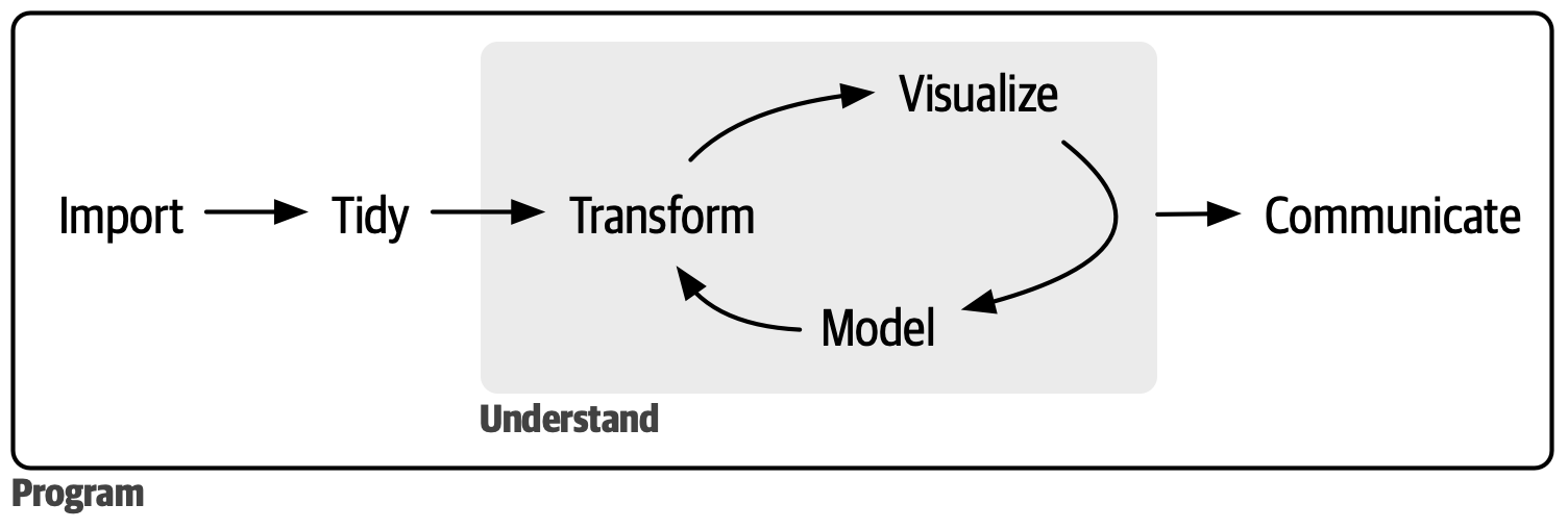
Recall - Data Science Workflow
Import
The data for this analysis comes courtesy of World Athletics, the world governing authority for athletics.
Complete event results from the past 7 Olympic games - from Atlanta 1996 to Tokyo 2020 - were acquired and paired with individual career progression data for every athlete who has competed during this span.
Career progression is defined as the top performances of an athlete in an event discipline from year to year throughout their career.
Import
This data set was then curated to identify and extract key factors and appropriately scale performances.
This is important because for Track events, one where the outcome is timed, lower is better, while for Field events, performances of larger magnitudes are preferred.
For convenience, athletes who competed in multiple individual events were separated into independent observations.
The analysis in this work is completely reproducible, with source code located at https://github.com/awosoga/peaks-and-primes.
Tidy
Results are taken from https://raw.githubusercontent.com/awosoga/peaks-and-primes/refs/heads/master/olympics_data.csv
olympics_results <- read_csv(olympic_results_url, show_col_types = F) %>%
  janitor::clean_names() %>%
  separate_wider_delim(date, delim = "–", names = c("start", "end")) %>%
  separate_wider_delim(cols = event,
                       names = c("gender", "event"), delim = " ",
                           too_many = "merge") %>%
  filter(str_detect(event, "Wheelchair", negate = T)) %>%
  mutate(# Manually fixed Aminata CAMARA's age
    birth_date = if_else(name == "Aminata CAMARA", "06 DEC 1973",
                         birth_date),
    gender = if_else(gender == "Men's", "Men", "Women"),
    across(c(birth_date, end),  ~as.Date(format(
    as.Date(., format = "%d %b %Y"), "%Y-%m-%d"))),
    age = year(end) - year(birth_date),
    ) %>% rename("nationality" = nat)
Tidy
Convert games to a factor with ordered levels, and create an event_category variable to distinguish between events.
olympics_results <- olympics_results %>%
  mutate(
    games = factor(games, ordered = T,
                        levels = c("The XXXII Olympic Games",
                                   "The XXXI Olympic Games",
                                   "The XXX Olympic Games",
                                   "The XXIX Olympic Games",
                                   "The XXVIII Olympic Games",
                                   "The XXVII Olympic Games",
                                   "The XXVI Olympic Games"),
                        labels = c("Tokyo '20", "Rio '16", "London '12",
                                   "Beijing '08", "Athens '04",
                                   "Sydney '00", "Atlanta '96")),
    event_category = if_else(
      str_detect(event, "Metres|Walk|Wheelchair") |
             event %in% c("Marathon"), "Track", "Field")) %>%
  mutate(event = if_else(event == "Javelin Throw (old)",
                         "Javelin Throw", event), games_year = year(end))
Tidy
Next, we create an event_type variable to categorize the events into meaningful groups.
olympics_results <- olympics_results %>%
  mutate(
    event_type = case_match(
      event,
      c("100 Metres", "200 Metres", "400 Metres", "400 Metres Hurdles",
        "100 Metres Hurdles", "110 Metres Hurdles") ~ "Sprints",
      c("800 Metres", "1500 Metres",
        "3000 Metres Steeplechase") ~ "Middle Distance",
      c("5000 Metres", "10,000 Metres") ~ "Long Distance",
      c("Heptathlon", "Decathlon") ~ "Combined Events",
      c("High Jump", "Long Jump", "Triple Jump", "Pole Vault") ~ "Jumps",
      c("Shot Put", "Discus Throw", "Hammer Throw",
        "Javelin Throw", "Javelin Throw (old)") ~ "Throws",
      c("10 Kilometres Race Walk", "20 Kilometres Race Walk",
        "50 Kilometres Race Walk", "Marathon") ~ "Road Races",
      .default = "Other"
    ))
Transform
Here, we load the career progression data and identify athletes who are still “active”. Career progression data can be found at https://raw.githubusercontent.com/awosoga/peaks-and-primes/refs/heads/master/career_progression.csv
Transform
We now begin a set of steps to find the season’s best performance of each athletes.
olympic_performances <- olympics_results %>%
  filter(!is.na(birth_date)) %>%
      distinct(birth_date, athlete_links, event, event_type,
               .keep_all = T) %>%
      select(name, birth_date, athlete_links, event, nationality,
             event_type, event_category, gender, games_year)

athlete_bests <-
  progression %>%  inner_join(olympic_performances,
    by = c("athlete_link" = "athlete_links", "event")
  ) %>%
  mutate(age_years = year(date) - year(birth_date),
         age_days = as.double(
           difftime(date, birth_date,units = "days")
           ),  # I will count hand timed results as legitimate
         performance = str_remove_all(performance, "h")
         )
Transform
Next, we convert the performance variable to a numeric value, accounting for the fact that track events are timed and field events are measured in distance or height.
athlete_bests <- athlete_bests %>%
    mutate(mark = if_else(
      event_category == "Track",
      as.numeric(
        difftime(
          parse_date_time2(performance,
                           orders = c("%H:%M:%S", "%M:%S:00",
                                      "%M:%OS", "%OS"),
                           exact = T),
          lubridate::parse_date_time2("0", orders ="S"),
          units = "secs"
        )
      ), parse_number(performance)),
      # the below accounts for edge cases like a 62s 400MH
      mark = if_else(is.na(mark), parse_number(performance), mark)
      )
Transform
We now have a data frame with the season’s best performances of each athlete.
athlete_bests <- athlete_bests %>%
    mutate(
      best_performance = case_when(
        # we want the lowest time
        event_category == "Track" & mark == min(mark, na.rm = T) ~ T,
        # we want the furthest/highest performance
        event_category == "Field" & mark == max(mark, na.rm = T) ~ T,
        .default = F
      ),
      percent_off_peak = if_else(event_category == "Track",
                                 abs((mark - min(mark, na.rm = T))/mark),
                                 abs((mark - max(mark, na.rm = T))/mark)),
      olympic_year = if_else(year %in% c(seq(1980, 2016, 4), 2021), T, F),
      .by = c("athlete_link", "event")
    ) %>%
  # remove duplicate seasons bests
  slice_max(with_ties = F, n = 1, order_by = age_days,
            by = c("event", "year",  "athlete_link"))
Summary Statistics
gender_ages_summary_statistics <-
olympics_results %>% group_by(games) %>%
  distinct(athlete_links, .keep_all = T) %>% ungroup() %>%
  summarise(mean = mean(age, na.rm = T), median = median(age, na.rm = T),
            sd = sd(age, na.rm = T), .by = "gender")

average_age <- olympics_results %>% group_by(games) %>%
  distinct(athlete_links, .keep_all = T) %>% ungroup() %>% pull(age) %>%
  mean(na.rm = T)

average_finalist_age <- olympics_results %>% group_by(games) %>%
  distinct(athlete_links, .keep_all = T) %>% ungroup() %>%
  filter(str_detect(event_meta, "Final")) %>%
  summarise(mean = mean(age, na.rm = T)) %>% pull()

average_medalist_age <- olympics_results %>%
  filter(str_detect(event_meta, "Final"), place %in% c(1:3)) %>%
  summarise(mean = mean(age, na.rm = T)) %>% pull()
Babe Wake Up, It’s an Olympic Year
It has been demonstrated that the ages of athletes at the Olympics in other sports such as gymnastics have experienced noticeable changes over time.
However, things have been remarkably consistent over the past 25 years in athletics, where the average age of just under 27 years old has displayed just 3 months of variation between Games.
The lone notable exception to this trend was Tokyo 2020, where the mean age of 27.6 years old is readily explained away by the 1 year delay of the Games due to the Covid-19 pandemic.
Babe Wake Up, It’s an Olympic Year
The overall mean ages are surprisingly similar between men and women as well (26.9 years old), though the median age of women is slightly higher (27 to 26).
Finalists were on average 16 months older than the average participant, but medalists were only 1 month older than average.
The standout example here was the 2008 Beijing Olympics, which recorded the lowest average medalist age of 26.1.
It is no coincidence that medalists from this Games included track legends Usain Bolt (22 years old), Shelly-Ann Fraser-Pryce (22 years old), and Allyson Felix (23 years old).
A Matter of Survival
Now that we are warmed up, we can go into more detail about the main engine used to investigate an athlete’s peak window in this work - survival analysis.
True to its name, survival analysis originated in studies of mortality among different demographics.
Its applications have since been generalized to study terminal events and the time until those events occur, with that event typically denoted as a failure (\(f\)) and survival time \(T\) considered as a random variable.
A Matter of Survival
The survival function \(S(t)\) gives the probability that a subject will survive past a given time \(t\):
\[ S(t) = \mathbb{P}(T > t) \]
\(S(t) \in [0,1]\) and in theory is smooth, though in reality is estimated from data as \(\hat{S}(t)\) using step functions.
A Matter of Survival
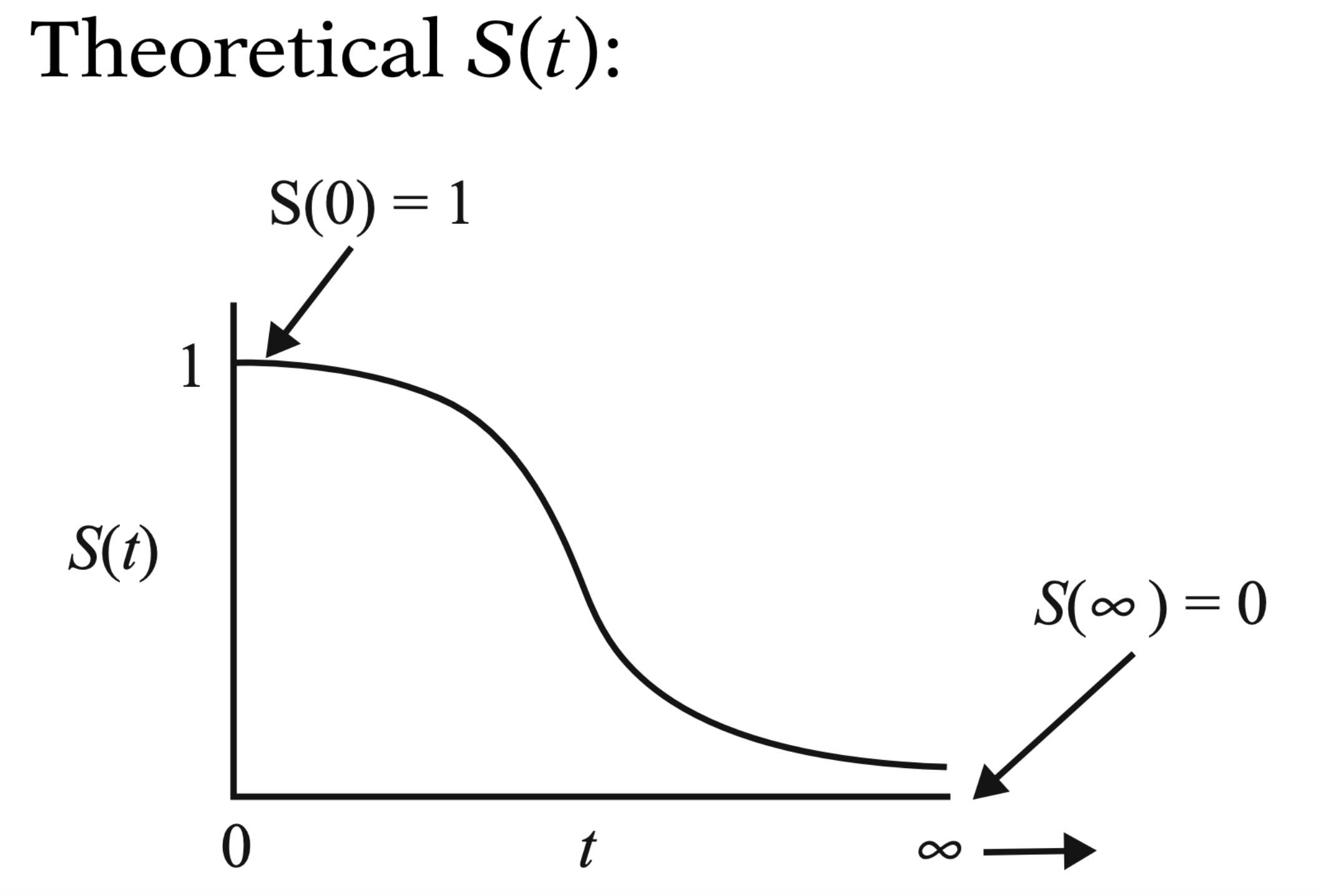
Theoretical Survival Curve
A Matter of Survival
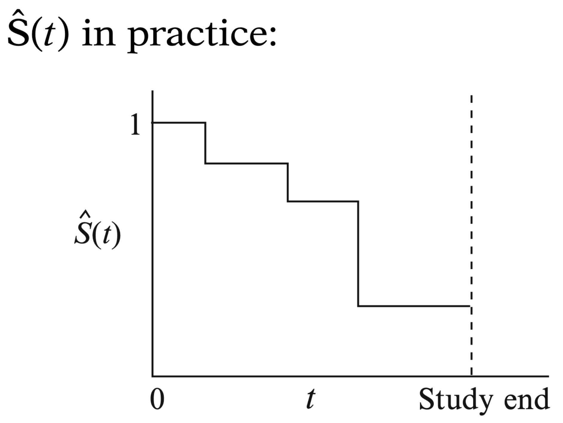
Estimated Survival Curve
A Matter of Survival
Our question is framed as “time until an athlete peaks”, where time is measured in years - the athlete’s age.
A key feature that distinguishes survival analysis from other methods is that the event of interest is not guaranteed to be observed in every entity when a study is completed. This can happen for example, if the study ends before the event occurs, or if the subject is lost to follow-up.
Special techniques are utilized to appropriately account for these types of observations.
A Matter of Survival
In our situation, an athlete’s peak cannot be definitively identified until their career has come to an end, so the active athletes in this data set are censored - given a special label to acknowledge their status.
We define \(d\) as a \((0,1)\) random variable that indicates either censorship or failure.
\[ d = \begin{cases} 1 & \text{if the athlete has peaked} \\ 0 & \text{if the athlete is still active} \\ \end{cases} \]
A Matter of Survival
Since it is unfeasible to manually validate the competing status of each athlete, a RETIRED label is given to athletes who do not have a recorded performance after December 31, 2022.
This definition falls short in edge cases where an athlete takes extended time off due to childbirth, a major injury, or to serve a suspension, for example, but the proportion of such athletes is assumed to be negligible.
A Matter of Survival
Here, we extract athlete personal bests and prepare the data for survival analysis.
athlete_peaks <- athlete_bests %>%
  filter(best_performance) %>%
    slice_max(n = 1, with_ties = F, order_by = age_days,
              by = c("event", "athlete_link")) %>%
  mutate(
    age_surv = Surv(age_years, retired == T),
    age_days_surv = Surv(age_days, retired == T),
  ) %>%
  mutate(across(c(nationality, gender, event_type,
                  event_category, olympic_year), factor))
Kaplan-Meier Curves
A Kaplan-Meier curve allows us to graph survival functions and estimate survival probability at a given time \(t\), defined as:
\[ \hat{S}(t) = \prod_{i: t_i \leq t} \left(1 - \frac{d_i}{n_i}\right) \]
where \(d_i\) is the number of failures at time \(t_i\), and \(n_i\) is the number of survivors (non-censored subjects) at time \(t_i\).
Kaplan-Meier Curves
Subsequently, we write;
\[ \hat{S}(t_{(f)}) = \prod^f_{i=1}\hat{Pr}[T > t_{(i)} | T \geq t_{(i)}] \\ = \hat{S}(t_{(f-1)}) \times \hat{Pr}(T > t_{(f)} | T \geq t_{(f)}) \]
This can be understood as the product of the survival estimate for the previous failure time multiplied by the conditional probability of surviving past the current failure time.
Visualize
Median values are typically used in place of averages in survival analysis because censored data are usually not normally distributed.
From the observed data, the median peak age is 27 years old, and this is illustrated visually via a Kaplan-Meier curve, where the probability of an athlete peaking dips under 50% for the first time after they turn 27.
The uncertainty estimates of these predictions are less than +/- 1% on average and can be viewed within the magnified portion of the visualization on the next page.
Visualize
km_curve_plot <-
  km_curve %>%
    ggsurvfit() +
    add_confidence_interval() +
    xlab("Age") + ylab("Probability of Peaking After A Given Age") +
    geom_point(aes(x = 27, y = 0.43857), size = 2, color = theme_color) +
    scale_y_continuous(labels = scales::percent) +
      geom_segment(aes(x = 27, y = -Inf, xend = 27, yend = 0.43857),
                   color = theme_color, linetype = "dashed" ) +
      geom_segment(aes(x = -Inf, y = 0.43857, xend = 27, yend = 0.43857),
                   color = theme_color, linetype = "dashed" ) +
      scale_x_continuous(breaks = c(seq(0, 20, 10), 27, seq(30, 50, 10)) ,
                         labels = as.character(
                           c(seq(0, 20, 10), 27, seq(30, 50, 10)))) +
      scale_y_continuous(breaks = c(0, 0.25, 0.44, 0.50, 0.75, 1),
                         labels = scales::percent)
Visualize
km_curve_plot <- km_curve_plot +
    theme(panel.grid.minor.y = element_blank(),
          panel.grid.minor.x = element_blank(),
           axis.text.x = element_text(
             face = ifelse(athlete_peaks$age_years ==27, "bold", "plain"),
             ),
          axis.text.y = element_text(
            face = c(rep("plain", 2), "bold", rep("plain", 2))
          )
          ) +
    ggmagnify::geom_magnify(
      from = c(xmin = 26, xmax = 29, ymin = 0.34, ymax = 0.54),
      to = c(xmin = 35, xmax = 45, ymin = 0.45, ymax = 0.95))

km_curve_plot
Visualize
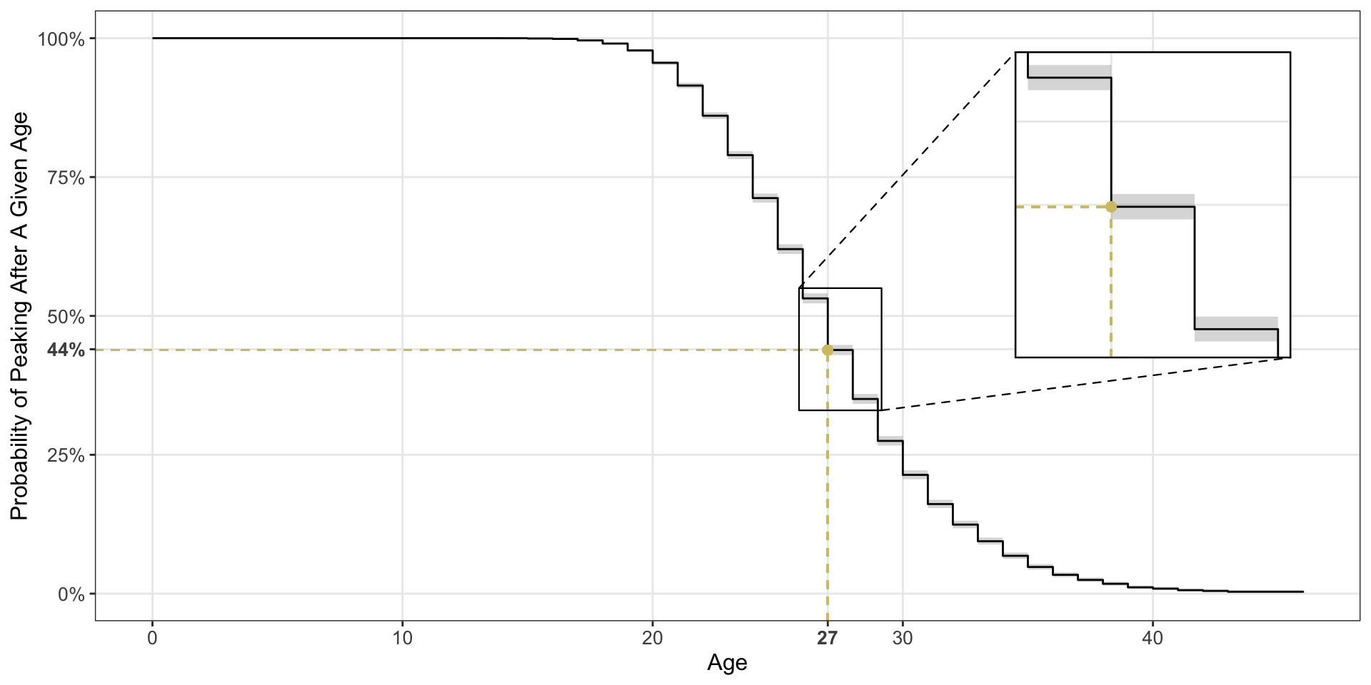
*A Kaplan-Meier curve allows us to estimate the probability that an athlete will peak after a given age. We use the curve by selecting a point of interest from the horizontal axis and locating the associated probability on the vertical axis. For example, the probability that an athlete peaks after 27 years old is 44%
Percent Off Peak
olympic_year_marks <- athlete_bests %>%
  filter(olympic_year) %>% pull(percent_off_peak)

non_olympic_year_marks <- athlete_bests %>%
  filter(!olympic_year) %>% pull(percent_off_peak)

ttest_results <- t.test(olympic_year_marks, non_olympic_year_marks)
ttest_results
    Welch Two Sample t-test

data:  olympic_year_marks and non_olympic_year_marks
t = -17.767, df = 60420, p-value < 2.2e-16
alternative hypothesis: true difference in means is not equal to 0
95 percent confidence interval:
 -0.007638189 -0.006120380
sample estimates:
 mean of x  mean of y
0.04461832 0.05149761
Percent Off Peak
This result is noteworthy as it implies that Olympic athletes are typically in their prime when they compete.
In fact, we see some indications of a relationship between the relative peaks in athlete performance and the years of Olympic Games, as the difference between an athlete’s proximity from their career best in Olympic years versus non Olympic years is statistically significant.
Although we have neither established the methodology necessary for appropriate causal analysis nor considered other factors such as injuries and World Championships, these preliminary results match our intuition about the incentive that the Games provide.
Keeping Up with the Times
An example of this is the 200m career progression of Tokyo 2020 Olympic Champion Andre De Grasse.
  athlete_bests %>%
  distinct(.keep_all = T) %>%
  filter(str_detect(athlete_link, "andre-de-grasse"),
         event == "200 Metres") %>%
  mutate(athlete = str_to_title(
    str_trim(str_replace_all(str_remove_all(
          str_extract(athlete_link, "[^/]+$"), "[0-9]"), "-", " ")))) %>%
  ggplot(aes(x = age_years, y = mark)) +
    geom_line() +
    geom_point(aes(color = olympic_year), size = 2, show.legend = F) +
    xlab("Age") +
    annotate("label", x = 22, y = 20.62, label = "Rio 2016",
             fontface = "bold", color = "white",  fill = theme_color) +
    annotate("label", x = 27, y = 20.62, label = "Tokyo 2020",
             fontface = "bold", color = "white", fill = theme_color) +
    ylab("Performance (s)") +
    scale_color_manual(values = c("black", theme_color)) +
    theme(panel.grid.major = element_blank())
Keeping Up with the Times
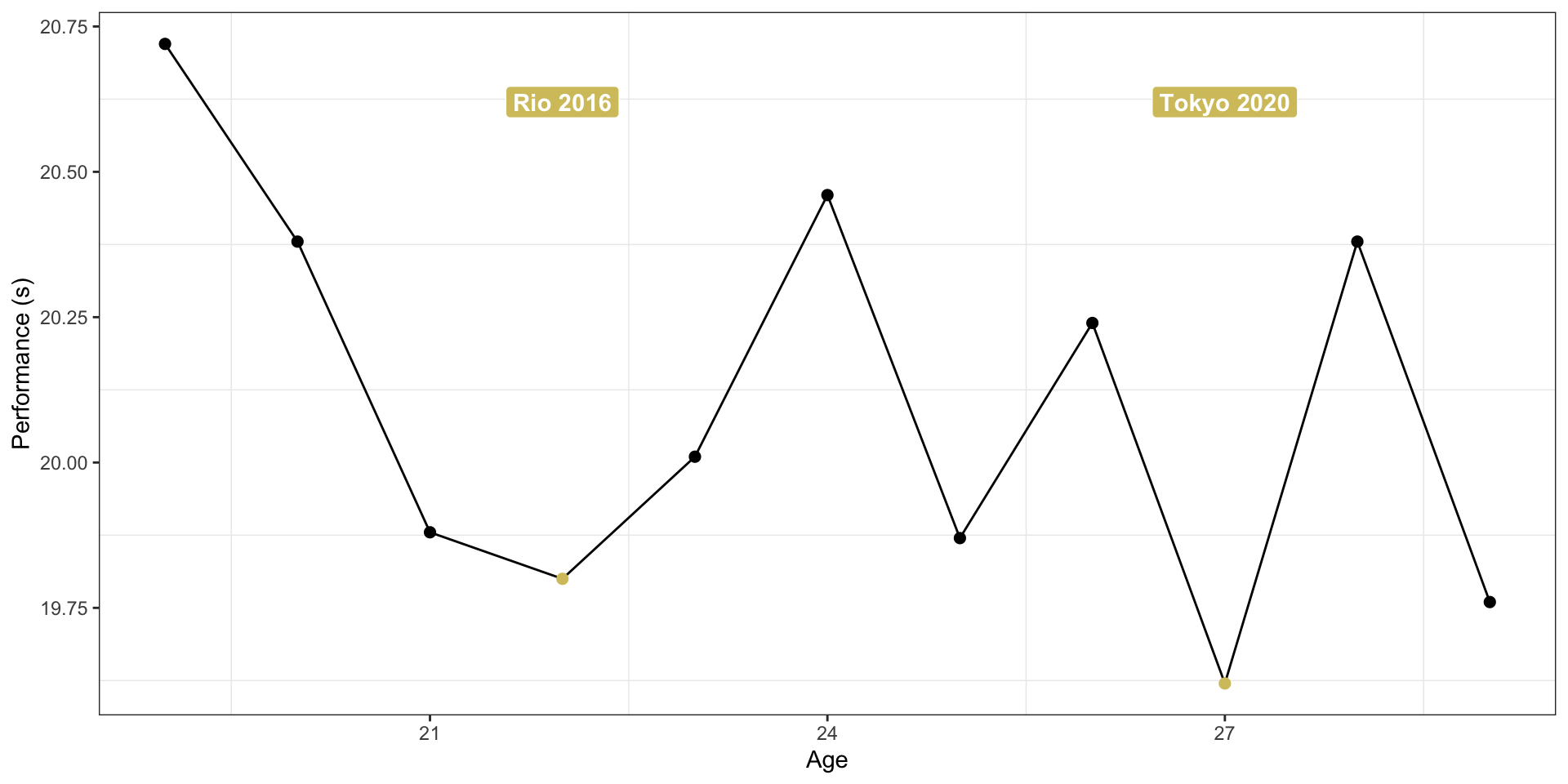
The career performance progression of Canadian sprinter Andre De Grasse in the 200m
Predicting the Peak
Unlike similar analyses that investigate athlete peaks from the lens of summary statistics and their confidence intervals, our approach allows us to build a model to identify certain factors that might predict an athlete’s peak.
A simple set of features was used in our final model:
gender,nationality,event type,a binary
olympic yearvariable, andtraining age.
Predicting the Peak
Training age is estimated as the number of years that an athlete has recorded an event performance at a World Athletics-sanctioned meet.
The rationale behind its inclusion is to try and capture the level of technical experience that an athlete has in their event.
This allows for differentiation between “late bloomers” (older athletes with a small training age) and “child prodigies” (younger athletes with a large training age).
Predicting the Peak
The selected model was an oblique random survival forest (Jaeger et al. 2024), which is an ensemble machine learning technique for modeling censored data.
It uses oblique (linear-combination) splits instead of axis-aligned (single-variable) splits, with improved efficiency over existing methods by exploiting various optimizations.
Additional design choices retain model interpretability, with predictive performance superior to many state of the art models.
It is implemented in R via the aorsf package (Jaeger et al. 2019)
Oblique Split Visualization
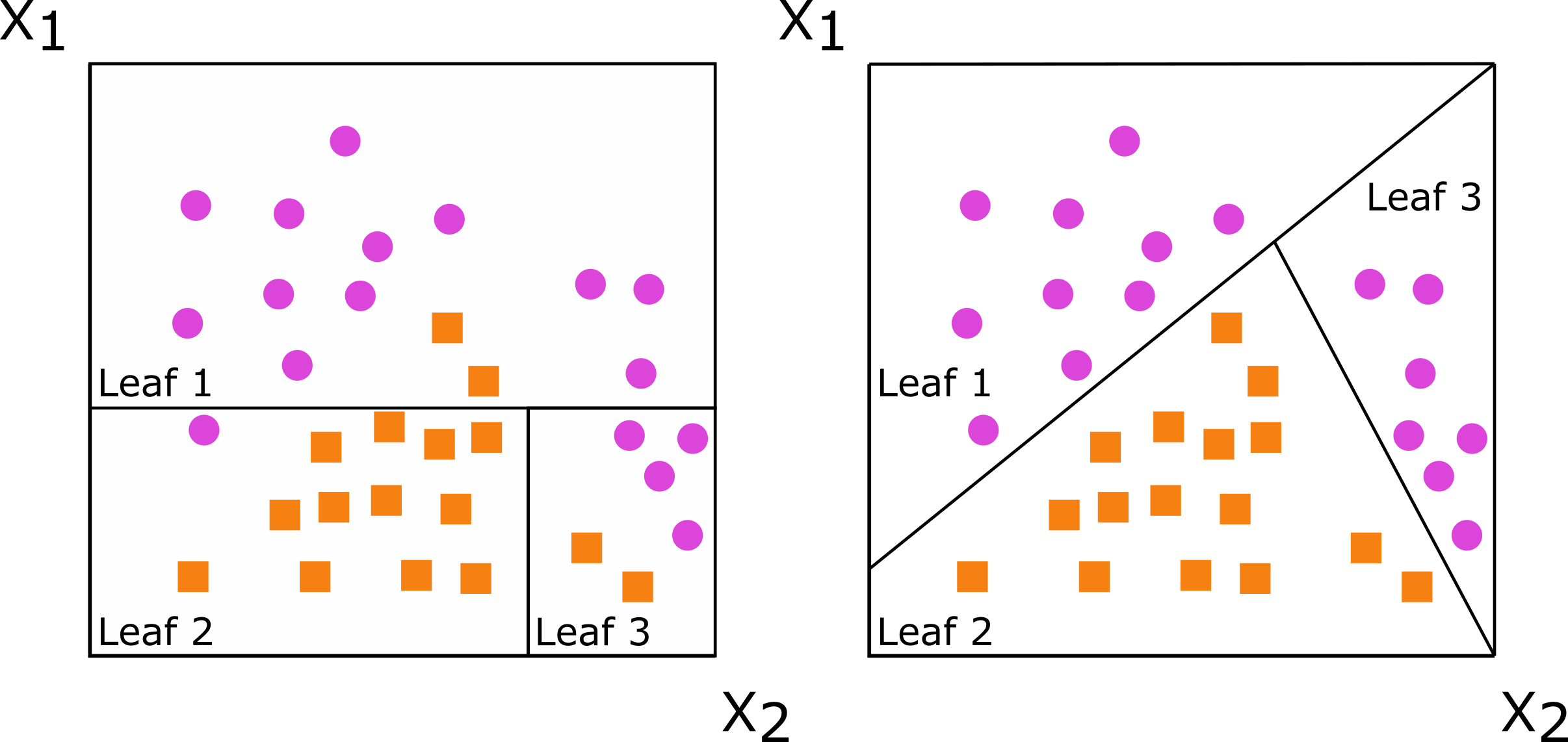
Figure: Decision trees for classification with axis-based splitting (left) and oblique splitting (right). Both trees partition the predictor space defined by variables X1 and X2, but the oblique splits do a better job of separating the two classes.
Oblique Split Visualization
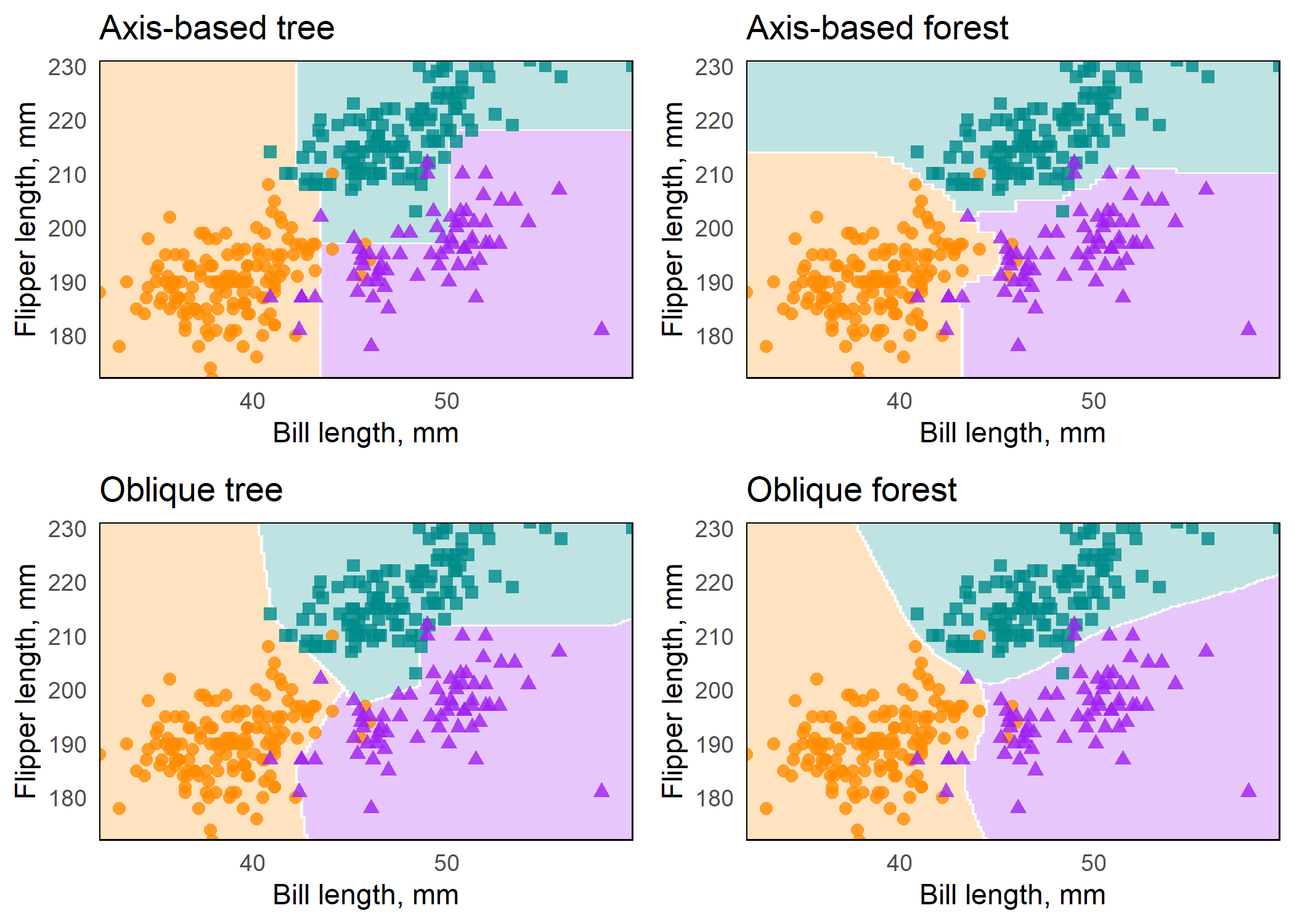
Figure: Axis-based and oblique decision surfaces from a single tree and an ensemble. Axis-based trees have boundaries perpendicular to predictor axes, whereas oblique trees can have boundaries that are neither parallel nor perpendicular to such axes.
Model
First, we split the data into training, validation, and test splits, and then define our model workflow.
set.seed(1)
peaks_split <- initial_validation_split(athlete_peaks)
peaks_train <- training(peaks_split)
peaks_rset <- validation_set(peaks_split)

model_recipe <- recipe(age_surv ~ nationality + gender + event_type +
                  olympic_year + training_age, data = athlete_peaks) %>%
  step_novel(nationality) %>% step_other(nationality, threshold = 0.001)

survival_metrics <- metric_set(brier_survival_integrated)
evaluation_time_points <- seq(0, 40, 1)

oblique_rsf <- rand_forest(mtry = tune(), min_n = tune()) %>%
  set_engine("aorsf") %>% set_mode("censored regression")

oblique_wflow <- workflow() %>% add_recipe(model_recipe) %>%
  add_model(oblique_rsf)
Model
Here is where we actually run the model
Model
Now we select the best hyperparameters and run the final model using them
param_best <- select_best(oblique_tuned,
                          metric = "brier_survival_integrated")
last_oblique_wflow <- finalize_workflow(oblique_wflow, param_best)

set.seed(2)
final_model <-
last_oblique_fit <- last_fit(
  last_oblique_wflow,
  split = peaks_split,
  metrics = survival_metrics,
  eval_time = evaluation_time_points,
)
Variable Importance
Now, we can analyze the contribution of each feature to the model via its variable importance, which in this context is ANOVA-based (Menze et al. 2011) - The importance of a variable is understood as the proportion of times that a variable has a statistically significant p-value when used in predictions.
Variable Importance
osrf_model <- final_model %>% extract_fit_engine()

osrf_model %>% orsf_vi() %>% enframe() %>%
  mutate(name = case_match(
    name, "event_type" ~ "event_category", .default = name),
    name = str_to_title(str_replace_all(name, "\\_", " "))) %>%
  ggplot(aes(x = reorder(name, value), y = value,
             label = round(value, 3))) +
  geom_col(fill = theme_color, color = "black") + coord_flip() +
  ylab("Variable Importance") + xlab("") +
  geom_text(position = position_dodge(width = 0.7),  hjust = 1.5,
            size = 6, fontface = "bold", color = "white") +
  theme_minimal() +
  theme(panel.grid = element_blank(), axis.text.x = element_blank())
Variable Importance
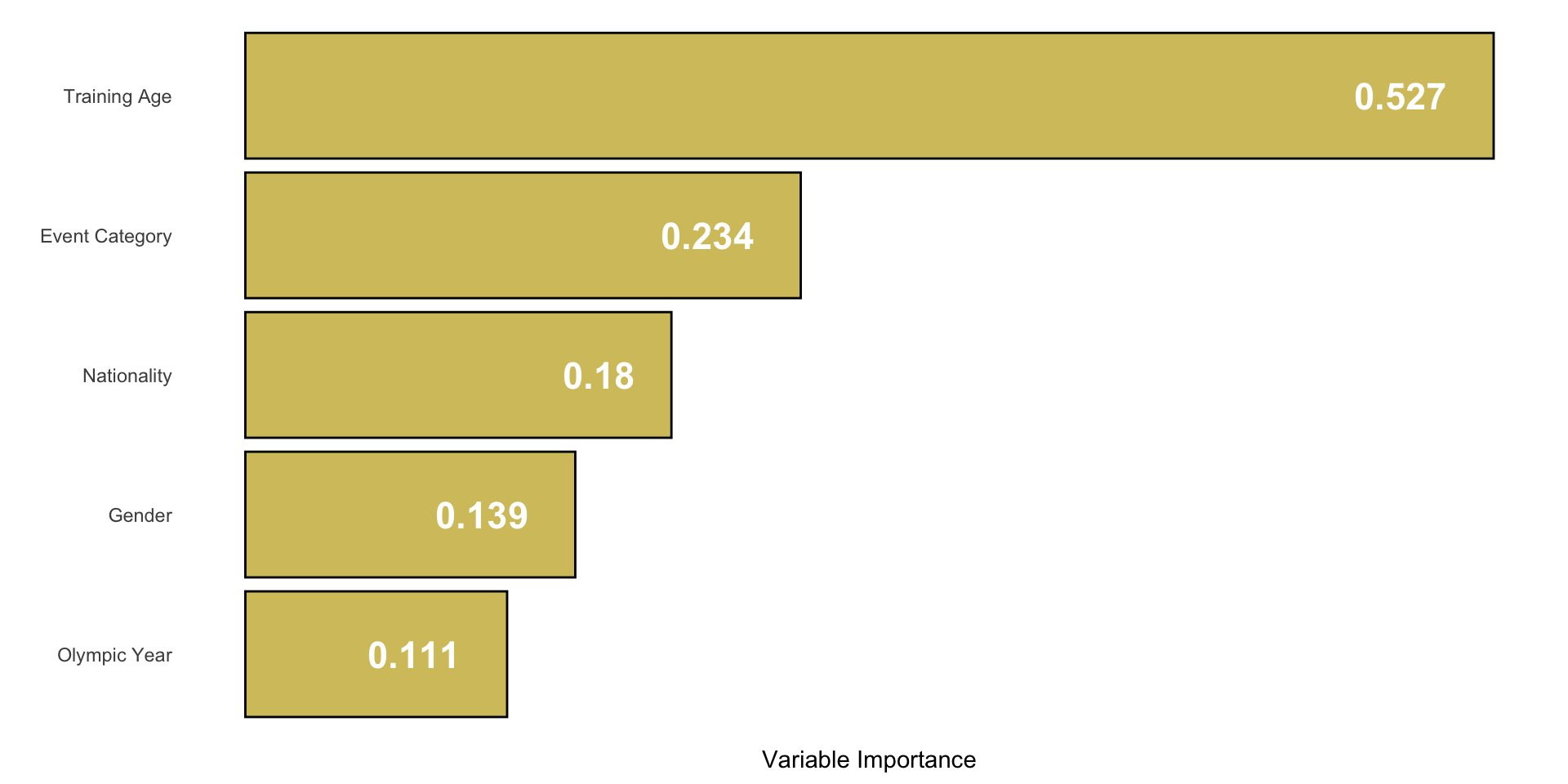
Quantifying Variable Importance
We see that
training ageis the most useful predictor of an athlete’s peak from our feature set.- This could be explained partially by the fact that it demonstrates some correlation with actual age, but also matches our intuition that “experience” does help predict peaks.
Event categoryhas the second-highest relative influence, and its overall score is computed as the average of the magnitudes from its subcategories.- Here, we see that the peaks of road racers are “easiest” to predict, while those of throwers are most difficult.
Quantifying Variable Importance
We hypothesize that the trend of older peaks in road racers improves the accuracy of model predictions, while finding out that Olympic throwers in our data set average the longest careers out of any event type may explain why peak age prediction is difficult for that event.
athlete_bests %>%
    slice_max(n = 1, with_ties = F, order_by = training_age,
              by = c(athlete_link, event)) %>%
    summarise(avg_career_length = mean(training_age),
              .by = "event_type") %>% gt() %>%
  fmt_number() %>%
  tab_header("Average Career Length by Event Type",
             subtitle = "Data taken from World Athletics") %>%
  gtExtras::gt_theme_538()
Quantifying Variable Importance
| Average Career Length by Event Type | |
|---|---|
| Data taken from World Athletics | |
| event_type | avg_career_length |
| Sprints | 11.64 |
| Road Races | 10.03 |
| Middle Distance | 11.49 |
| Jumps | 13.57 |
| Long Distance | 9.89 |
| Throws | 13.93 |
| Combined Events | 10.71 |
Quantifying Variable Importance
The relative importance of
nationalitycomes as a bit of a surprise, though we speculate that it requires further decomposition in order to make inferences on its various subcomponents.Genderhas the second smallest variable importance of the feature set, and the predicted differences in example tests is quite small.Finally, we find evidence that knowledge of an
Olympic yeardoes indeed help predict if an athlete will peak, though this is by far the least impactful feature.
The Curious Case of Kim Collins
Differences between predicted values and the realized data can be interpreted in terms of athletes who peak earlier or later than expected, which serves as an interesting case study.
However, there is a lot of noise near the extreme values of this continuum, likely confounded by the unconventional means by which many of the identified athletes were selected for an Olympic Games.
Filtering out this noise unearths a remarkable outlier, 5-time Olympian Kim Collins of St. Kitts and Nevis.
The Curious Case of Kim Collins
oldest_peaks <- athlete_peaks %>%
  filter(event_type != "Road Races") %>%
  select(year, nationality, event, performance,
         name, age_years, age_days) %>%
  slice_max(n = 5, order_by = age_days) %>%
  mutate(name = str_to_title(name),
         nationality = case_match(
           nationality,
           "SKN" ~ "KNA",
           "BER" ~ "BMU",
           "GER" ~ "DEU",
           .default = nationality
         )) %>%
  left_join(countrypops %>%
              distinct(country_name, country_code_2, country_code_3),
            by = c("nationality" = "country_code_3"))
The Curious Case of Kim Collins
oldest_peaks %>%
  gt() %>%
  gtExtras::gt_theme_nytimes() %>%
  tab_header("Oldest Peaks Among Olympians Since 1996",
             subtitle = "Excluding road racers.
             Data taken from World Athletics") %>%
  tab_style(
    style = list(cell_fill(color= "#FF000070")),
    locations = cells_body(
        columns = everything(),
        rows = name == "Kim Collins"
  )) %>% cols_label(age_years = "Age", country_code_2 = "Nationality") %>%
      fmt_flag(columns = country_code_2) %>%
  fmt_country(columns = nationality) %>%
    cols_hide(c(country_name, age_days)) %>%
  cols_merge(c(country_code_2, nationality)) %>%
  cols_move_to_start(c(year, country_code_2, nationality))
The Curious Case of Kim Collins
| Oldest Peaks Among Olympians Since 1996 | |||||
|---|---|---|---|---|---|
| Excluding road racers. Data taken from World Athletics | |||||
| year | Nationality | event | performance | name | Age |
| 2012 | Ukraine | Hammer Throw | 79.42 | Oleksandr Dryhol | 46 |
| 2006 | Russia | 100 Metres | 11.18 | Irina Khabarova | 40 |
| 2016 | St. Kitts & Nevis | 100 Metres | 9.93 | Kim Collins | 40 |
| 2012 | Azerbaijan | Hammer Throw | 79.56 | Dmitriy Marshin | 40 |
| 2000 | United Kingdom | Discus Throw | 65.08 | Robert Weir | 39 |
Model Predictions
predictions <- athlete_peaks %>% bind_cols(
  predict(extract_workflow(final_model),
          new_data = athlete_peaks, type = "time"))
kim_collins_100 <-
predictions %>% mutate(age_diff = .pred_time - age_years) %>%
  filter(str_detect(athlete_link, "kim-collins"),
         event == "100 Metres") %>%
  select(event, performance, age_years, .pred_time, age_diff)
The correlation between training age and the age of peak performance among retired athletes is found below
The Curious Case of Kim Collins
The 2003 World Champion’s personal best in the 100m of 9.93 seconds came at age 40, a whopping 13 years after his predicted peak age of 27.
This is tied for the second-oldest peak among non-road racers in the entire data set, trailing only Oleksandr Dryhol’s 79.42m hammer throw at the age of 46 - a mark set a few months before a retroactive ban from London 2012 for prohibited substance use.
The Curious Case of Kim Collins
One thing to consider, however, is that the average retirement age for athletes in our data set is 32 years old.
While this speaks volumes to Collins’ longevity, it also means that his peak is only comparable to a small subset of eligible athletes who were active at similar ages.
Nevertheless, Collins’ career progression is particularly noteworthy because he seemingly experienced two primes, one between 2002 and 2005 (ages 26-29), and another from 2013 to 2016 (ages 37-40).
The Curious Case of Kim Collins
In fact, each of Collins’ 4 best seasons came during the window of his “second prime”, as shown in the image below.
athlete_bests %>% filter(str_detect(athlete_link, "kim-collins"),
         event == "100 Metres", age_years> 21) %>%
  mutate(career_type = if_else(year %in% c(2002:2005, 2013:2016),
                               "prime", "normal")) %>%
  ggplot(aes(x = year, y = mark, label = age_years)) +
  annotate("label", x = 2003.5, y = 9.94, label = "Prime #1",
           fill = theme_color, color = "white", fontface = "bold") +
  annotate("label", x = 2014.5, y = 10.02, label = "Prime #2",
           color = "white", fill = theme_color, fontface = "bold") +
  geom_line() +
  geom_point(aes(color = career_type), size = 7, show.legend = F) +
  geom_text(color = "white", fontface = "bold") +
  scale_y_continuous(labels = function(x) sprintf("%.2f", x),
                     breaks = seq(9.90, 10.45, 0.05)) +
  xlab("Year") + ylab("Performance (s)") +
  scale_color_manual(values = c("black", theme_color)) +
  theme(panel.grid.major.x = element_blank(),
        panel.grid.minor.x = element_blank())
The Curious Case of Kim Collins
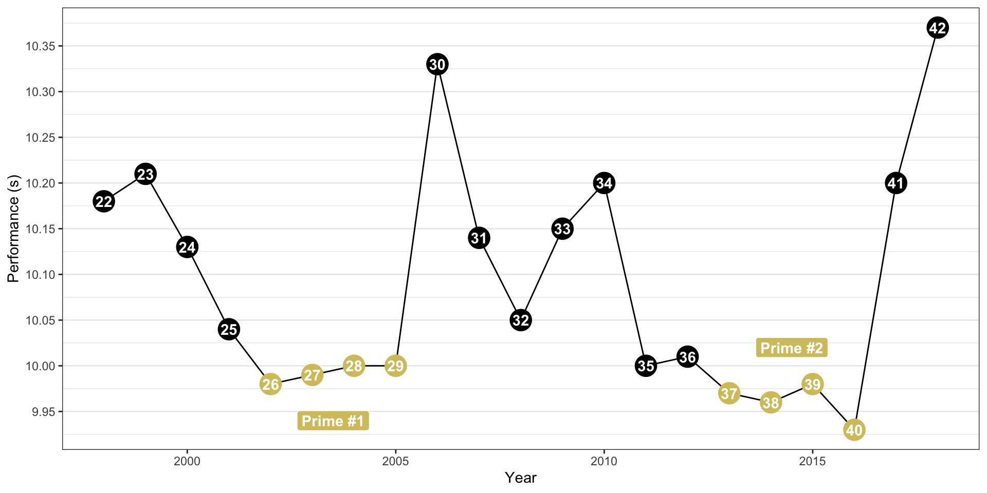
The career progression of Kim Collins in the 100m from age 22 onwards
Conclusion
By leveraging survival analysis, we were able to make meaningful predictions about the age at which Olympic track and field athletes peak.
We also find that the prime of a track and field athlete typically spans a single Olympic games, though some athletes such as Kim Collins seem to have experienced multiple windows.
Conclusion
We found that the training age of an athlete was the most influential predictor of peak age, while the timing of the Olympics and the athlete’s nationality, event category, gender were less informative.
By investigating these physiological and external factors, we gain a greater appreciation for the uphill battle that athletes face as they prepare themselves for what will most likely be their only chance at attaining Olympic glory.
Extensions
Including an additional feature to capture how an athlete qualifies for the Olympic Games, such as a proxy for the relative depth of an athlete’s NOC or their proximity to entry standards, could be incredibly valuable.
Implementing a more rigorous methodological treatment to athletes who compete in multiple individual events may remove bias from the model.
Further analysis on the rate of progression leading up to and following an athlete’s peak could be used to identify athletes who have a slow and steady progression versus a sharp ascension followed by a rapid decline.
Acknowledgement
This work was made possible through collaboration within the University of Waterloo Analytics Group for Games and Sports (UWAGGS). A special thanks goes to member Rithika Silva for his extensive support with data acquisition.
References
Discussion Questions
Assignment 6
What is something new that you learned from the readings this week?
What is something that you had already interacted with in a previous class?
What is something that you would like clarification on or like to see expanded upon?
Any comments from the assignment questions?
Next Up
- Module 3: Development Operations (DevOps)
- DO4DS Chapters 13-18
- Assignment 7: Due July 2 @ 11 AM on Crowdmark
Appendix: A Crash Course on Tree-Based Methods
STAT 441/841 will cover this information in much greater detail.
Description
Tree-based methods can be used in many supervised learning problems.
Since they do not assume a specific functional form between predictors and the response variable, they can capture complex interactions and nonlinearities in the data.
They have a plethora of application areas, including in feature selection, classification and regression problems, and survival analysis.
Their true strengths arise when they are utilized in ensemble methods, where the predictions of numerous trees are strategically combined to improve predictive results.
Summary
The information included here is adapted from “Introduction to Statistical Learning: With Examples in R” textbook by James et al. (2021) and “Applied Statistical Learning” by Schonlau (2023).
Decision Trees
Decision trees are quite primitive but make up the foundation of many more complex methods.
They are defined by using a series of “if-then” statements called “splits” to recursively partition the data into subsets based on the values of predictor variables.
Splits are chosen based on a criteria to minimize error or maximize information gain.
The tree structure allows for easy interpretation and visualization, as each internal node represents a decision based on a predictor variable, and each leaf node represents a final prediction.
Bagging
An issue with individual decision trees is the high variance of their estimates.
We can use the well known bootstrap technique (Efron 1979) to reduce this variance by taking the average predictions of many trees built using boostrapped samples of the training data.
This is known as bootstrap aggregation, from which bagging derives its name (Breiman 1996).
Bagging
Bagging is a general purpose method useful across different statistical learning techniques, but is particularly useful for tree-based methods.
Due to its bootstrapped construction, it is very straightforward to estimate test error, called out-of-bag (OOB) error, without needing to resort to more computationally expensive methods such as cross-validation.
Random Forests
Random forests (Breiman 2001) extend upon bagging with a small but essential modification to drastically reduce the correlation found between trees.
Instead of building decision trees using the same number of predictors at each split, random forests select a random sample of predictors at each split, which means that trees will look quite different from one another.
Random Forests
This heterogeneity further improves the variance reduction achieved by bagging, while maintaining higher levels of interpretability.
This is particularly useful with high-dimensional data where the number of predictors is large relative to the number of observations, as it allows for more robust predictions without overfitting.
Examples
Consider the classification problem where we use the iris dataset and want to predict the species of flower based on various measurements.
Decision Trees
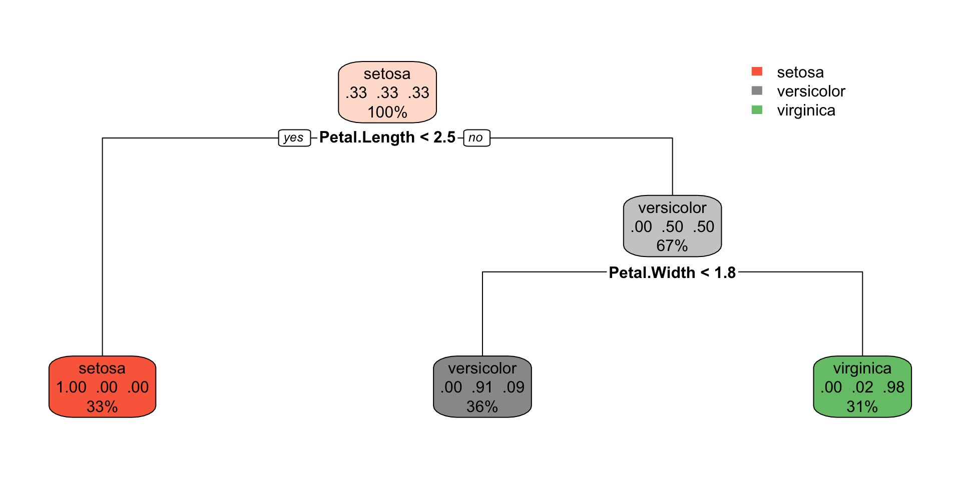
- Choose the best feature to split: We evaluate splits based on a chosen criterion like Gini impurity (Ceriani and Verme 2012; Breiman et al. 2017) or information gain (Quinlan 1986; Shannon, n.d.)
- We find that the best initial split for the data is on a
Petal.Lengthof 2.5 cm. By doing so we are able to classify all flowers that have a petal length of less than 2.5 cm assetosa.
Decision Trees
- To differentiate between
virginicaandversicolor, we find that the next best split is onPetal.Width. We see that we are able to almost perfectly classify all flowers with a petal width of less than 1.8 cm asversicolor, and flowers with a petal width of more than 1.8 cm asvirginica. - We could continue to add more depth to the tree until we were able to perfectly differentiate the flower types, but these gains are deemed marginal by the splitting criterion and therefore we stop here.
Bagging
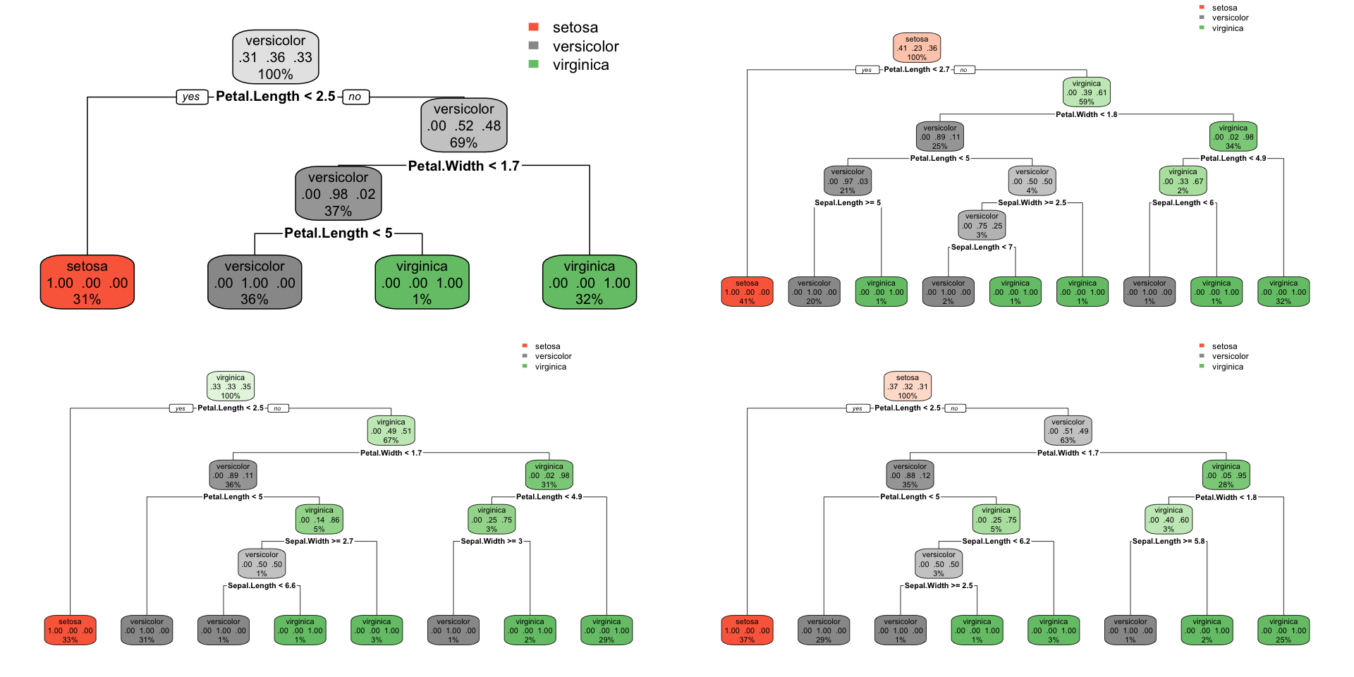
We consider the same classification problem with the iris dataset, but instead use bagging. Here, we
Bagging
- Randomly sample the observations (with replacement) to create \(B\) different data sets.
- We would then train \(B\) decision trees, each on one of those data sets.
Bagging
- As shown in the visualization with \(B=4\) bootstrapped samples, the data (and corresponding splits) are all slightly different, and for a given combination of covariates each tree makes a prediction.
- The final output is the majority vote of the predctions from each tree since we are doing classification (it would be the average predicted value if we were doing regression).
Random Forest
We follow the same procedure as in bagging, but instead of considering all 4 covariates as candidates for splitting the tree as shown in the previous example, we make each split using \(p < 4\) covariates (i.e. 2) as candidates.
With \(B = 25\) trees, we have an out-of-bag error rate of 4.67%, which is an improvement on the 6% OOB error of bagging with the same number of replications.

STAT 468 - Introductory Sports Performance Analysis